(New page: == Original MATLAB code == After running the original program through MATLAB, the following plot was producted:) |
|||
| (3 intermediate revisions by the same user not shown) | |||
| Line 1: | Line 1: | ||
| − | + | After running the given MATLAB code, the following plot was produced: | |
| − | + | ||
| + | [[Image:Orig plot_ECE301Fall2008mboutin.png]] | ||
| + | |||
| + | As seen above, the picture does not resemble a 13Hz sinusoidal wave repeated 13 times. The function that was suppose to be plotted by the code should be | ||
| + | |||
| + | <math>\,x(t)=Re[e^{j(2\pi F_{o}t-\frac{pi}{2})}]\,</math> | ||
| + | |||
| + | <math>\,x(t)=Re[cos(2\pi F_{o}t-\frac{pi}{2})+jsin(2\pi F_{o}t-\frac{pi}{2})]\,</math> | ||
| + | |||
| + | <math>\,x(t)=cos(2\pi F_{o}t-\frac{pi}{2})\,</math> | ||
| + | |||
| + | which appears to be correct. However, the sampling period <math>T_{s}=0.07</math> only provides 14 points on the graph, which appears to be not enough. If we increase the number of sampling points by a factor of 10 (with a new value <math>T_{s}=0.007</math>), the following plot is produced: | ||
| + | |||
| + | [[Image:Jkubasci Fixed plot_ECE301Fall2008mboutin.png]] | ||
| + | |||
| + | This looks correct. Thus, the problem was not with the code, but with the sampling period chosen. The value <math>T_{s}=0.07</math> roughly sampled one point from each period of the sinusodial wave, which was not fine enough to describe the wave sufficiently. | ||
Latest revision as of 17:53, 11 September 2008
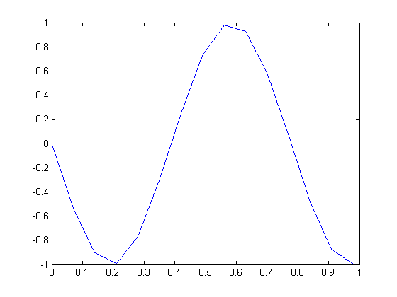
After running the given MATLAB code, the following plot was produced:
As seen above, the picture does not resemble a 13Hz sinusoidal wave repeated 13 times. The function that was suppose to be plotted by the code should be
$ \,x(t)=Re[e^{j(2\pi F_{o}t-\frac{pi}{2})}]\, $
$ \,x(t)=Re[cos(2\pi F_{o}t-\frac{pi}{2})+jsin(2\pi F_{o}t-\frac{pi}{2})]\, $
$ \,x(t)=cos(2\pi F_{o}t-\frac{pi}{2})\, $
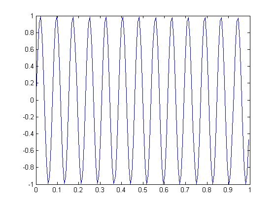
which appears to be correct. However, the sampling period $ T_{s}=0.07 $ only provides 14 points on the graph, which appears to be not enough. If we increase the number of sampling points by a factor of 10 (with a new value $ T_{s}=0.007 $), the following plot is produced:
This looks correct. Thus, the problem was not with the code, but with the sampling period chosen. The value $ T_{s}=0.07 $ roughly sampled one point from each period of the sinusodial wave, which was not fine enough to describe the wave sufficiently.


