(New page: ==Fixing the Bug== The problem with the code provided was that the sampling rate was much too large for the function in question. With the sampling rate this low, it is impossible to get a...) |
(→Fixing the Bug) |
||
| (One intermediate revision by the same user not shown) | |||
| Line 2: | Line 2: | ||
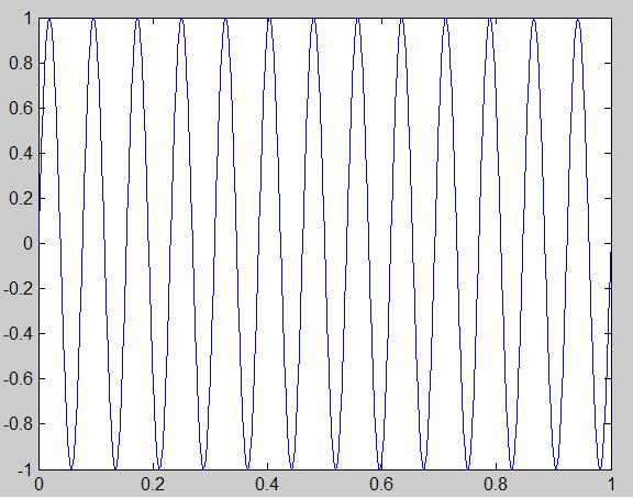
The problem with the code provided was that the sampling rate was much too large for the function in question. With the sampling rate this low, it is impossible to get an accurate representation of what the function actually looks like. To fix this problem, just decrease the time between samples (Ts). As shown below, I chose a Ts value of 0.001. It provided a resolution fine enough to easily observe what the function is supposed to look like. | The problem with the code provided was that the sampling rate was much too large for the function in question. With the sampling rate this low, it is impossible to get an accurate representation of what the function actually looks like. To fix this problem, just decrease the time between samples (Ts). As shown below, I chose a Ts value of 0.001. It provided a resolution fine enough to easily observe what the function is supposed to look like. | ||
| − | < | + | <pre> |
%Ben Moeller | %Ben Moeller | ||
%Fixing the bug | %Fixing the bug | ||
| Line 18: | Line 18: | ||
plot(t,x) | plot(t,x) | ||
</pre> | </pre> | ||
| + | |||
| + | |||
| + | [[Image:hw2a_moellerb_ECE301Fall2008mboutin.jpg|300px|frame|center|13 Cycles of the Signal]] | ||
Latest revision as of 09:31, 11 September 2008
Fixing the Bug
The problem with the code provided was that the sampling rate was much too large for the function in question. With the sampling rate this low, it is impossible to get an accurate representation of what the function actually looks like. To fix this problem, just decrease the time between samples (Ts). As shown below, I chose a Ts value of 0.001. It provided a resolution fine enough to easily observe what the function is supposed to look like.
%Ben Moeller
%Fixing the bug

F0 =13;

T0 =1/F0

Ts = 0.001;

t  = 0:Ts:13*T0

x = real(exp(j*(2*pi*F0*t-pi/2)));

plot(t,x)


