| Line 181: | Line 181: | ||
Properties of the pmf: <br/> | Properties of the pmf: <br/> | ||
1. (proof)<br/> | 1. (proof)<br/> | ||
| − | <center><math>P_X(x) \ | + | <center><math>P_X(x) \geq 0</math></center> |
| − | 2. (proof | + | 2. (proof)<br/> |
<center><math>\sum_{x\in\mathcal R}P_X(x) = 1</math></center> | <center><math>\sum_{x\in\mathcal R}P_X(x) = 1</math></center> | ||
Revision as of 05:42, 3 October 2013
Random Variables and Signals
Topic 6: Random Variables: Distributions
How do we find , compute and model P(x ∈ A) for a random variable X for all A ∈ B(R)? We use three different functions:
- the cumulative distribution function (cdf)
- the probability density function (pdf)
- the probability mass function (pmf)
We will discuss these in this order, although we could come at this discussion in a different way and a different order and arrive at the same place.
Definition $ \quad $ The cumulative distribution function (cdf) of X is defined as
Notation $ \quad $ Normally, we write this as
So $ F_X(x) $ tells us P$ P_X(A) $ if A = (-∞,x] for some real x.
What about other A ∈ B(R)? It can be shown that any A ∈ B(R) can be written as a countable sequence of set operations (unions, intersections, complements) on intervals of the form (-∞,x$ _n $], so can use the probability axioms to find $ P_X(A) $ from $ F_X $ for any A ∈ B(R). This is not how we do things in practice normally. This will be discussed more later.
Can an arbitrary function $ F_X, $ be a valid cdf? No, it cannot.
Properties of a valid cdf:
1.
This is because
and
2. For any $ x_1,x_2 $ ∈ R such that $ x_1<x_2 $,
i.e. $ F_X(x) $ is a non decreasing function.
3. $ F_X $ is continuous from the right , i.e.
Proof:
First, we need some results from analysis and measure theory:
(i) For a sequence of sets, $ A_1, A_2,... $, if $ A_1 $ ⊃ $ A_2 $ ⊃ ..., then
(ii) If $ A_1 $ ⊃ $ A_2 $ ⊃ ..., then
(iii) We can write $ F_X(x^+) $ as
Now let
Then
4. $ P(X>x) = 1-F_X(x) $ for all x ∈ R
5. If $ x_1 < x_2 $, then
6. $ P(\{X=x\})= F_X(x) - F_X(x^-) $, where
Contents
The Probability Density Function
Definition $ \quad $ The probability density function (pdf) of a random variable X is the derivative of the cdf of X,
at points where $ F_x $ is differentiable.
From the Fundamental Theorem of Calculus, we then have that
Important note: the cdf $ F_X $ might not be differentiable everywhere. At points where $ F_X $ is not differentiable, we can use the Dirac delta function to defing $ f_x $.
Definition $ \quad $ The Dirac Delta Function $ \delta(x) $ is the function satisfying the properties:
1.
2.
If $ F_X $ is not differentiable at a point, use $ \delta(x) $ at that point to represent $ f_X $.
Why do we do this? Consider the step function $ u(x) $, which is discontinuous and thus not differentiable at $ x=0 $. This is a common type of discontinuity we see in cdfs. The derivative of $ u(x) $ is defined as
This limit does not exist at $ x=0 $
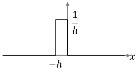
Let's look at the function
It looks like this:
For any x ≠ 0, we have that
for small enough h.
Also, ∀ $ \epsilon $<0,
So, in the limit, the function g(x) has the properties of the $ \delta $-function as h tends to 0. A similar argument can be made for h<0.
So this is why it is sometimes written that
Since we will only work with non-differentiable functions that have step discontinuities as cdfs, we write
with the understanding that $ d/dx $ is not necessarily the traditional definition of the derivative.
Properties of the pdf:
1. (proof)
2. (proof)
3. (proof) if $ x_1<x_2 $, then
Some notes:
- We introduced the concept of a pdf in our discussion of probability spaces. We could have defined the pdf of a random variable X as a function $ f_X $ satisfying properties 1 and 2 above, and then define $ F_X $ in terms of $ f_X $.
- f_X(x) is not a probability for a fixed x, it gives us instead the "probability density", so it must be integrated to give us the probability.
- In practice, to compute probabilities of random variable X, we normally use
Continuous and Discrete Random Variables
A random variable X having a cdf that is continuous everywhere is called a continuous random variable.
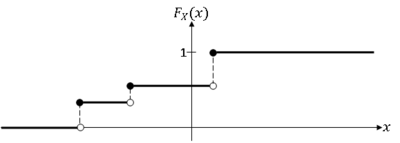
A random variable X having a piece-wise constant cdf is a discrete random variable.
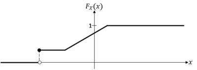
A random variable X whose cdf is neither continuous everywhere nor piece-wise constant is a mixed random variable.
We will consider only discrete and continuous random variables in this course.
Note:
- For a continuous random variable X, P(X=x)=0 ∀x ∈ R, because <mathF_X(x)-F_X(x^-) = 0</math> ∀x ∈ R.
- We can use the cdf/pdf functions for a discrete random variable X, but generally, we do not. Instead, we use the pmf.
Probability Mass Function
The probability mass function (pmf) of random variable X is the function
We will use this function when X is discrete.
Although P(X=x) exists for every x ∈ R, we normally define $ p_X(x) $ for some subset R⊂R
Definition $ \quad $ Given random variable X:S→R, let R = X(S) be the range space of X (note that the range of X is still R).
Example: Let X be the sum of values rolled on two fair die. Then R = {2,3,...,12}.
We define the pmf only on R, so in the example above, we would have $ P_X(x) = P(X=x) $ ∀x ∈ R.
We can now consider the probability space for a discrete random variable to be (R,P(R),P$ _X $).
Note that if X is continuous, we define the cdf/pdf for all x ∈ R. for example, if X = V</math>^2</math>, where V is the voltage (so X is proportional to power), then R=[0,∞), but we still define $ f_X(x) $ ∀x ∈ R.
Properties of the pmf:
1. (proof)
2. (proof)
These properties can be derived from the axioms. Note that we could simple define the pmf to be a function having these two and then create a probability mapping P(.) in such a way that P(.) will satisfy the axioms. We discussed this in our lectures on probability spaces. This is what we do in practice.
References
- M. Comer. ECE 600. Class Lecture. Random Variables and Signals. Faculty of Electrical Engineering, Purdue University. Fall 2013.


