(New page: [Category:ECE600]] Category:Lecture notes <center><font size= 4> '''Random Variables and Signals''' </font size> <font size= 3> Topic 8: Functions of Random Variables</font size> </c...) |
|||
| Line 1: | Line 1: | ||
| − | [Category:ECE600]] | + | [[Category:ECE600]] |
[[Category:Lecture notes]] | [[Category:Lecture notes]] | ||
Revision as of 09:10, 11 October 2013
Random Variables and Signals
Topic 8: Functions of Random Variables
We often do not work with the random variable we observe directly, but with some function of that random variable. So, instead of working with a random variable X, we might instead have some random variable Y=g(X) for some function g:R → R.
In this case, we might model Y directly to bet f$ _Y $(y), especially if we do not know g. Or we might have a model for X and find f$ _Y $(y) (or p$ _Y $(y)) as a function of f$ _X $ (or p$ _X $ and g.
We will discuss the latter approach here.
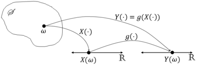
More formally, let X be a random variable on (S,F,P) and consider a mapping g:R → R. Then let Y$ (\omega)= $g(X($ \omega)) $ ∀$ \omega $ ∈ S.
We normally write this as Y=g(X).
Graphically,
Is Y a random variable? We must have Y$ ^{-1} $(A) ≡ {$ \omega $ ∈ S: Y$ (\omega) $ ∈ A} = {$ \omega $ ∈ S: g(X$ (\omega) $) ∈ A} be an element of F ∀A ∈ B(R) (Y must be Borel measurable).
We will only consider functions g in this class for which Y$ ^{-1} $(A) ∈ F ∀A ∈ B(R), so that if Y=g(X) for some random variable X, Y will be a random variable.
What is the distribution of Y? Consider 3 cases:
- X discrete, Y discrete
- X continuous, Y discrete
- X continuous, Y continuous
Note: you cannot have a continuous Y from a discrete X.
Case 1: X & Y discrete
Let $ R_X $≡ X(S) be the range space of X and math>R_Y</math>≡ g(X(S)) be the range space of Y. Then the pmf of Y is
But this means that
Example $ \quad $ Let X be the value rolled on a die and
Then R$ _X $ = {0,1,2,3,4,5,6} and R$ _Y $ = {0,1} and g(x) = x % 2.
Now
Case 2: X continuous, Y discrete
The pmf of Y in this case is


