(New page: Category:ECE600 Category:Lecture notes Back to all ECE 600 notes <center><font size= 4> '''Random Variables and Signals''' </font size> <font size=...) |
|||
| Line 27: | Line 27: | ||
Note that | Note that | ||
| − | * X(t,< | + | * X(t,<math>\omega</math>) (or simply X(t)) is a random process. |
| − | * X(t<math>_0</math>,< | + | * X(t<math>_0</math>,<math>\omega</math>) is a random variable for fixed t<math>_0</math>. |
| − | * X(t,< | + | * X(t,<math>\omega_0</math>) is a real-valued function of t for fixed <math>\omega_0</math>. |
| − | * X(t<math>_0</math>,< | + | * X(t<math>_0</math>,<math>\omega_0</math>) is a real number for fixed t<math>_0<math> and <math>\omega_0</math>. |
There are four types or random processes we will consider | There are four types or random processes we will consider | ||
| Line 38: | Line 38: | ||
# T ⊂ '''R''' countable, X(t) a continuous random variable for every t ∈ T is a '''discrete-time continuous random process'''. | # T ⊂ '''R''' countable, X(t) a continuous random variable for every t ∈ T is a '''discrete-time continuous random process'''. | ||
| − | '''Example''' <math>\qquad</math> if T = '''N''' = {1,2,3,...}, then X(t) is a discrete time random process, usually written as X<math> | + | '''Example''' <math>\qquad</math> if T = '''N''' = {1,2,3,...}, then X(t) is a discrete time random process, usually written as X<math>_1</math>,X<math>_2</math> |
'''Example''' <math>\qquad</math> a binary waveform with random transition times | '''Example''' <math>\qquad</math> a binary waveform with random transition times | ||
| Line 44: | Line 44: | ||
<center>[[Image:fig2_stochastic_processes.png|350px|thumb|left|Fig 2: A binary waveform with random transition times.]]</center> | <center>[[Image:fig2_stochastic_processes.png|350px|thumb|left|Fig 2: A binary waveform with random transition times.]]</center> | ||
| + | |||
'''Example''' <math>\qquad</math> A sinusoid with random frequency <br/> | '''Example''' <math>\qquad</math> A sinusoid with random frequency <br/> | ||
Revision as of 08:44, 25 November 2013
Random Variables and Signals
Topic 19: Stochastic Processes
Stochastic Processes
We have already seen discrete-time random processes, but we will now formalize the concept of random process, including both discrete-time and continuous time.
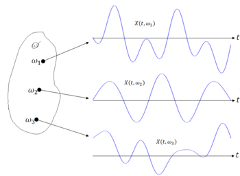
'Definition $ \qquad $ a stochastic process, or random process, defines on (S,F,P) is a family of random variables {X(t), t ∈ T} indexed by a set T.
Each waveform is referred to as a sample realization. Note that T can be uncountable, as shown above, or countable.
Note that
- X(t,$ \omega $) (or simply X(t)) is a random process.
- X(t$ _0 $,$ \omega $) is a random variable for fixed t$ _0 $.
- X(t,$ \omega_0 $) is a real-valued function of t for fixed $ \omega_0 $.
- X(t$ _0 $,$ \omega_0 $) is a real number for fixed t$ _0<math> and <math>\omega_0 $.
There are four types or random processes we will consider
- T ⊂ R uncountable, X(t) a discrete random variable for every t ∈ T is a continuous-time discrete random process.
- T ⊂ R uncountable, X(t) a continuous random variable for every t ∈ T is a continuous time continuous random process.
- T ⊂ R countable, X(t) a discrete random variable for every t ∈ T is a discrete-time discrete random process.
- T ⊂ R countable, X(t) a continuous random variable for every t ∈ T is a discrete-time continuous random process.
Example $ \qquad $ if T = N = {1,2,3,...}, then X(t) is a discrete time random process, usually written as X$ _1 $,X$ _2 $
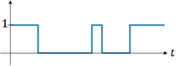
Example $ \qquad $ a binary waveform with random transition times
Example $ \qquad $ A sinusoid with random frequency
where $ \Omega $ is a random variable.
Probabilistic Description of a Random Process
We can use joint pdfs of pmfs, but often we use the first and second order moments instead.


