| Line 56: | Line 56: | ||
We can use joint pdfs of pmfs, but often we use the first and second order moments instead. | We can use joint pdfs of pmfs, but often we use the first and second order moments instead. | ||
| + | |||
| + | '''Definition''' <math>\qquad</math> The '''nth order cdf''' of X(t) is <br/> | ||
| + | <center><math>F_{X(t_1)...X(t_n)}(x_1,...,x_n)\equiv P(X(t_1)\leq x_1,...,X(t_n)\leq x_n)</math></center> | ||
| + | and the '''nth order pdf''' is <br/> | ||
| + | <center><math>f_{X(t_1)...X(t_n)}(x_1,...,x_n)=\frac{\partial F_{X(t_1)...X(t_n)}(x_1,...,x_n)}{\partial x_1...\partial x_n}</math></center> | ||
| + | |||
| + | '''Notation''' <math>\qquad</math> for n=1, we have <br/> | ||
| + | <center><math>f_{X(t_1)}(x_1)=f_{X_1}(x_1)</math></center> | ||
| + | and for n= 2, <br/> | ||
| + | <center><math>f_{X(t_1)X(t_2)}(x_1, x_2)=f_{X_1X_2}(x_1,x_2)</math></center> | ||
| + | |||
| + | '''Definition''' <math>\qquad</math> The '''nth order pmf''' of a discrete random process is <br/> | ||
| + | <center><math>p_{X(t_1)...X(t_n)}(x_1,...,x_n)=P(X(t_1)=x_1,...,X(t_n)=x_n)</math></center> | ||
| + | |||
| + | It can be shown that if f<math>_{X(t1)...X(tn)}</math>(x<math>_1</math>,...x<math>_n</math>) is specified ∀t<math>_1</math>,...,t<math>_n</math>; ∀n = 1,2,..., then X(t) is a valid random process consistent with a probability space (''S,F'',P). This result comes from the Kolmogorov existence theorem, which we will not cover. | ||
| + | |||
| + | Now consider the first and second order moments for a random process. | ||
| + | |||
| + | '''Definition''' <math>\qquad</math> The '''mean of a random process''' X(t) is <br/> | ||
| + | <center><math>\mu_X(t)\equiv E[X(t)]\quad\forall t\in T</math></center> | ||
| + | |||
| + | '''Definition''' <math>\qquad</math> The '''autocorrelation function''' of a random process X(t) is <br> | ||
| + | <center><math>R_{XX}(t_1,t_2)\equiv E[X(t_1)X(t_2)]</math></center> | ||
| + | Note: R<math>_{XX}</math>(t<math>_1</math>,t<math>_2</math>) = R<math>_{XX}</math>(t<math>_2</math>,t<math>_1</math>) | ||
| + | |||
| + | '''Definition''' <math>\qquad</math> The '''autocovariance function''' of a random process X(t) is <br> | ||
| + | <center><math>\begin{align} | ||
| + | C_{XX}(t_1,t_2)&\equiv E[(X(t_1)-\mu_X(t_1))(X(t_2)-\mu_X(t_2))] \\ | ||
| + | &=R_{XX}(t_1,t_2)-\mu_X(t_1)\mu_X(t_2) | ||
| + | \end{align}</math></center> | ||
| + | |||
| + | |||
| + | Important property of R<math>_{XX}</math> and C<math>_{XX}</math>: <br/> | ||
| + | R<math>_{XX}</math> and C<math>_{XX}</math> are non-negative definite functions, i.e., ∀a<math>_1</math>,...,a<math>_n</math> ∈ '''R''' and t<math>_1</math>,...,t<math>_n</math> ∈ '''R''', and ∀n ∈ '''N''', <br/> | ||
| + | <center><math>\sum_{i=1}^n\sum_{j=1}^na_ia_jR_{XX}(t_1,t_j)\geq 0</math></center> | ||
| + | |||
| + | '''Proof''' <math>\qquad</math> See the proof of NND property of correlation matrix R<math>_X</math>. Let R<math>_{ij}</math> = R<math>_{XX}</math>(t<math>_i</math>, t<math>_j</math>). | ||
| + | |||
| + | |||
| + | Two important properties of random processes: | ||
| + | |||
| + | '''Definition''' <math>\qquad</math> A random process W(t) is called a '''white noise process''' if C<math>_{WW}</math>(t<math>_1</math>,t<math>_2</math>) = 0 ∀t<math>_1</math> ≠ t<math>_2</math>. | ||
| + | |||
| + | This means that ∀t<math>_1</math> ≠ t<math>_2</math>, W(t<math>_1</math>) and W(t<math>_2</math>) are uncorrelated. | ||
| + | |||
| + | '''Definition''' <math>\qquad</math> A random process X(t) is called a '''Gaussian random process''' if X(t<math>_1</math>),...,X(t<math>_n</math>) are jointly Gaussian random variables ∀t<math>_1</math>,...,t<math>_n</math> for any n ∈ '''N'''. | ||
| + | |||
| + | |||
| + | The nth order characteristic function of a Gaussian random process is given by <br/> | ||
| + | <center><math>\Phi_{X(t_1)...X(t_n)}(\omega_1,...,\omega_n) = e^{ i\sum_{k=1}^n \mu_X(t_k)\omega_k - \frac{1}{2} \sum_{j=1}^n \sum_{k=1}^n C_{XX}(t_j,t_k)\omega_j\omega_k}</math></center> | ||
| + | |||
| + | |||
| + | ---- | ||
| + | |||
| + | ==Stationarity== | ||
| + | |||
| + | Intuitive idea: A random process is stationary (is some sense) if its probabilistic description (nth order cdf/pdf/pmf, or mean, autocorrelation, autocovariance functions) does not depend on the time origin. | ||
| + | |||
| + | |||
| + | <center>[[Image:fig3_stochastic_processes.png|350px|thumb|left|Fig 3]]</center> | ||
| + | |||
| + | Does the nth order cdf/pdf/pmf depend on where t=0 is? Do <math>\mu_X</math>(t), R<math>_{XX}</math>(t<math>_1</math>,t<math>_2</math>), C<math>_{XX}</math>(t<math>_1</math>,t<math>_2</math>)? | ||
| + | |||
| + | '''Defintion''' <math>\qquad</math> a random process X(tO is '''stict sense stationary (SSS)''', or simply '''stationary''', if <br/> | ||
| + | <center><math>F_{X(t_1)...X(t_n)}(x_1,...,x_n)=F_{X(t_1+\alpha)...X(t_n+\alpha)}(x_1,...,x_n)</math><br/> | ||
| + | <math>\forall\alpha\in\mathbb R,\;n\in\mathbb N,\;t_1,...,t_n\in\mathbb R</math></center> | ||
Revision as of 20:09, 30 November 2013
Random Variables and Signals
Topic 19: Stochastic Processes
Stochastic Processes
We have already seen discrete-time random processes, but we will now formalize the concept of random process, including both discrete-time and continuous time.
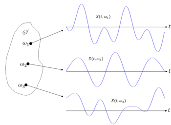
'Definition $ \qquad $ a stochastic process, or random process, defines on (S,F,P) is a family of random variables {X(t), t ∈ T} indexed by a set T.
Each waveform is referred to as a sample realization. Note that T can be uncountable, as shown above, or countable.
Note that
- X(t,$ \omega $) (or simply X(t)) is a random process.
- X(t$ _0 $,$ \omega $) is a random variable for fixed t$ _0 $.
- X(t,$ \omega_0 $) is a real-valued function of t for fixed $ \omega_0 $.
- X(t$ _0 $,$ \omega_0 $) is a real number for fixed t$ _0<math> and <math>\omega_0 $.
There are four types or random processes we will consider
- T ⊂ R uncountable, X(t) a discrete random variable for every t ∈ T is a continuous-time discrete random process.
- T ⊂ R uncountable, X(t) a continuous random variable for every t ∈ T is a continuous time continuous random process.
- T ⊂ R countable, X(t) a discrete random variable for every t ∈ T is a discrete-time discrete random process.
- T ⊂ R countable, X(t) a continuous random variable for every t ∈ T is a discrete-time continuous random process.
Example $ \qquad $ if T = N = {1,2,3,...}, then X(t) is a discrete time random process, usually written as X$ _1 $,X$ _2 $
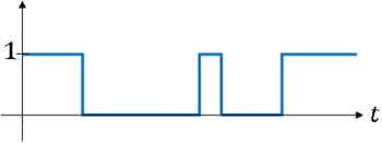
Example $ \qquad $ a binary waveform with random transition times
Example $ \qquad $ A sinusoid with random frequency
where $ \Omega $ is a random variable.
Probabilistic Description of a Random Process
We can use joint pdfs of pmfs, but often we use the first and second order moments instead.
Definition $ \qquad $ The nth order cdf of X(t) is
and the nth order pdf is
Notation $ \qquad $ for n=1, we have
and for n= 2,
Definition $ \qquad $ The nth order pmf of a discrete random process is
It can be shown that if f$ _{X(t1)...X(tn)} $(x$ _1 $,...x$ _n $) is specified ∀t$ _1 $,...,t$ _n $; ∀n = 1,2,..., then X(t) is a valid random process consistent with a probability space (S,F,P). This result comes from the Kolmogorov existence theorem, which we will not cover.
Now consider the first and second order moments for a random process.
Definition $ \qquad $ The mean of a random process X(t) is
Definition $ \qquad $ The autocorrelation function of a random process X(t) is
Note: R$ _{XX} $(t$ _1 $,t$ _2 $) = R$ _{XX} $(t$ _2 $,t$ _1 $)
Definition $ \qquad $ The autocovariance function of a random process X(t) is
Important property of R$ _{XX} $ and C$ _{XX} $:
R$ _{XX} $ and C$ _{XX} $ are non-negative definite functions, i.e., ∀a$ _1 $,...,a$ _n $ ∈ R and t$ _1 $,...,t$ _n $ ∈ R, and ∀n ∈ N,
Proof $ \qquad $ See the proof of NND property of correlation matrix R$ _X $. Let R$ _{ij} $ = R$ _{XX} $(t$ _i $, t$ _j $).
Two important properties of random processes:
Definition $ \qquad $ A random process W(t) is called a white noise process if C$ _{WW} $(t$ _1 $,t$ _2 $) = 0 ∀t$ _1 $ ≠ t$ _2 $.
This means that ∀t$ _1 $ ≠ t$ _2 $, W(t$ _1 $) and W(t$ _2 $) are uncorrelated.
Definition $ \qquad $ A random process X(t) is called a Gaussian random process if X(t$ _1 $),...,X(t$ _n $) are jointly Gaussian random variables ∀t$ _1 $,...,t$ _n $ for any n ∈ N.
The nth order characteristic function of a Gaussian random process is given by
Stationarity
Intuitive idea: A random process is stationary (is some sense) if its probabilistic description (nth order cdf/pdf/pmf, or mean, autocorrelation, autocovariance functions) does not depend on the time origin.
Does the nth order cdf/pdf/pmf depend on where t=0 is? Do $ \mu_X $(t), R$ _{XX} $(t$ _1 $,t$ _2 $), C$ _{XX} $(t$ _1 $,t$ _2 $)?
Defintion $ \qquad $ a random process X(tO is stict sense stationary (SSS), or simply stationary, if
$ \forall\alpha\in\mathbb R,\;n\in\mathbb N,\;t_1,...,t_n\in\mathbb R $


