ECE600 F13 Random Vectors mhossain - Rhea

Topic 17: Random Vectors

Random Vectors

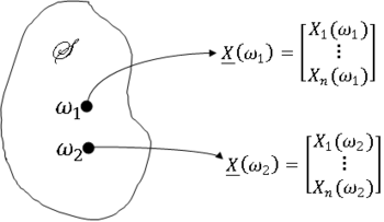
Definition $\qquad$ let X $$ _1 $$ ,..., X $$ _n $$ be n random variables on (S,F,P). The column vector X is given by

\underline{X} = [X_1,...,X_n]^T

is a random vector (RV) on (S,F,P).

Fig 1: The mapping from the sample space to the event space under X

$ _j $

.

We can view X( $\omega$ ) as a point in R $$ ^n $$ ∀ $\omega$ ∈ S.
Much of what we need to work with random vectors we can get by a simple extension of what we have developed for n = 2.

For example:

The cumulative distribution function of X is

F_{\underline X}(\underline x) = P(X_1\leq x_1,...,X_n\leq x_n)\;\;\forall\underline x = [x_1,...,x_n]^T\in\mathbb R^n

and the probability density function of X is

f_{\underline X}(\underline x) = \frac{\partial^nF_{\underline X}(\underline x)}{\partial x_1...\partial x_n}

For any D ⊂ R $$ ^n $$ such that D ∈ B(R $$ ^2 $$ ),

P(\underline X \in D) = \int_D f_{\underline X}(\underline x)d\underline x

Note that B(R

$ ^n $

) is the

\sigma

-field generated by the collection of all open n-dimensional hypercubes (more formally, k-cells) in R

$ ^n $

.

The formula for the joint pdf of two functions of two random variables can be extended to find the pdf of n functions of n random variables (see Papoulis).

The random variables X $$ _1 $$ ,..., X $$ _n $$ are statistically independent if the events {X $$ _1 $$ ∈ A $$ _1 $$ },..., {X $$ _n $$ ∈ A $$ _n $$ } are independent ∀A $$ _1 $$ , ..., A $$ _n $$ ∈ B(R). An equivalent definition is that X $$ _1 $$ ,..., X $$ _n $$ are independent if

f_{\underline X}(\underline x)=\prod_{i=1}^nf_{X_i}(x_i)\;\;\forall\underline x\in\mathbb R^n

Random Vectors: Moments

We will spend some time on moments of random vectors. We will be especially interested in pairwise covariances/correlations.
The correlation between X $$ _j $$ and X $$ _k $$ is denoted R $_{jk}$ , so

R_{jk} \equiv E[X_jX_k]

and the covariance is C $_{jk}$ :

C_{jk}\equiv E[(X_j-\mu_{X_j})(X_k-\mu_{X_k})]

For a random vector X, we define the correlation matrix R_X as

R_{\underline X}=\begin{bmatrix} R_{11} & \cdots & R_{1n} \\ \vdots & & \vdots \\ R_{n1} & \cdots & R_{nn} \end{bmatrix}

and the covariance matrix C_X as

C_{\underline X}=\begin{bmatrix} C_{11} & \cdots & C_{1n} \\ \vdots & & \vdots \\ C_{n1} & \cdots & C_{nn} \end{bmatrix}

The mean vector $\mu$ _X is

\mu_{\underline X}=[\overline X_1,\cdots,\overline X_n]^T

Note that the correlation matrix and the covariance matrix can be written as

\begin{align} R_{\underline X}&=E[\underline X\underline X^T] \\ C_{\underline X}&=E[(\underline X-\mu_{\underline X})(\underline X-\mu_{\underline X})^T] \end{align}

Note that $\mu$ _X, R_X and C_X are the moments we most commonly use for the random vectors.

We need to discuss an important property of R_X, but first, a definition from Linear Algebra.

Definition $\qquad$ An n × m matrix B with b $_{ij}$ as its i,j $^{th}$ entry is non-negative definite (NND) (or positive semidefinite) if

\sum_{i=1}^n\sum_{j=1}^n x_i x_j b_{ij} \geq 0

for all real vectors [x $$ _1 $$ ,...,x $$ _n $$ ] ∈ R $$ ^n $$ .

That is to say that for any real vector x, the product x $$ ^T $$ Ax, where A is a real matrix, is non negative.

Theorem $\qquad$ For any random vector X, R_X is NND.

Proof: $\qquad$ let a be an arbitrary real vector in R $$ ^n $$ , and let

Y = \underline a^T\underline X = \underline X^T\underline a

be a scalar random variable. Then

\begin{align}0\leq E[Y^2]&=E[\underline a^T\underline X\underline X^T\underline a] \\ &=\underline a^TE[\underline X\underline X^T]\underline a \\ &=\underline a^TR_{\underline X}\underline a \end{align}

So

0\leq \underline a^TR_{\underline X}\underline a = \sum_{i=1}^n\sum_{j=1}^na_ia_jR_{ij}

and thus, R_X is NND

Note: C_X is also NND.

Characteristic Functions of Random Vectors

Definition $\qquad$ let X be a random vector on (S,F,P). Then the characteristic function of X is

\Phi_{\underline X}(\underline\Omega)=E\left[e^{i\sum_{j=1}^n\omega_jX_j}\right]

where

\underline\Omega = [\omega_1,...,\omega_n]^T \in \mathbb R^n

The characteristic function Φ_X is extremely useful for finding pdfs of sums of random variables.
Let

Z=\sum_{j=1}^nX_j

Then

\Phi_Z(\omega)=E\left[e^{i\omega\sum_{j=1}^nX_j}\right] = \Phi_{\underline X}(\omega,...,\omega)

If X $$ _1 $$ ,..., X $$ _n $$ are independent, then

\Phi_Z(\omega)=\prod_{j=1}^n\Phi_{X_j}(\omega)

If, in addition, X $$ _1 $$ ,..., X $$ _n $$ are identically distributed with common characteristic function Φ $$ _X $$ , then

\Phi_Z(\omega) = (\Phi_X(\omega))^n \

Gaussian Random Vectors

Definition $\qquad$ Let X be a random vector on (S,F,P). Then X is Gaussian and X $$ _1 $$ ,..., X $$ _n $$ are said to be jointly Gaussian iff

Z=a_0+\sum_{j=1}^na_jX_j

is a Gaussian random variable ∀[a $$ _0 $$ ,..., a $$ _n $$ ] ∈ R $^{n+1}$ .

Now we will show that the characteristic function of a Gaussian random vector X is

\Phi_{\underline X}(\underline\Omega) = e^{i\underline\Omega^T\mu_{\underline X}-\frac{1}{2}\underline\Omega^TC_{\underline X}\underline\Omega^T}

where $\mu$ _X is the mean vector of X and C_X is the covariance matrix.

Proof $\qquad$ Let

Z = \sum_{j=1}^n\omega_jX_j

for

\underline\Omega \in \mathbb R^n

Then Z is a Gaussian random variable since X is Gaussian. So

\Phi_Z(\omega)=e^{i\omega\mu_Z}e^{-\frac{1}{2}\omega^2\sigma_Z^2}

where

\begin{align} \mu_Z&=E\left[\sum_{j=1}^n\omega_jX_j\right] \\ &=\sum_{j=1}^n\omega_j\mu_{X_j} \\ &=\underline\Omega^T\mu_{\underline X} \end{align}

and

\begin{align} \sigma_Z^2 &= \mbox{Var}\left(\sum_{j=1}^n\omega_jX_j\right) \\ &= \sum_{j=1}^n\sum_{k=1}^n\sigma_{jk}\omega_j\omega_k \\ &=\underline\Omega^TC_{\underline X}\underline\Omega \end{align}

where

\sigma_{jk}^2 = E[(X_j-\mu_{X_j})(X_k-\mu_{X_k})]

and C_X is the covariance matrix of X.

Now

\begin{align} \Phi_{\underline X}(\omega)&= E\left[e^{i\sum_{j=i}^n\omega_jX_j}\right] \\ &= \Phi_Z(\omega) \end{align}

Plugging the expressions for $\mu_Z$ and $\sigma_Z$ $$ ^2 $$ into Φ $$ _Z $$ gives

\Phi_{\underline X}(\omega) =e^{i\underline\Omega^T\mu_{\underline X}}e^{-\frac{1}{2}\underline\Omega^TC_{\underline X}\underline\Omega}

Note that we can use the equation

f_{\underline X}(\underline x) = \frac{1}{(2\pi)^n}\int_{\mathbb R^n}\Phi_{\underline X}(\underline\Omega)e^{-i\underline\Omega^T\underline x}d\underline\Omega

to show that if X is Gaussian, then

f_{\underline X}(\underline x) = \frac{1}{\sqrt{(2\pi)^n|C_{\underline X}|}}e^{-\frac{1}{2}(\underline X-\mu_{\underline X})^TC_{\underline X}^{-1}(\underline X-\mu_{\underline X})}

\forall \underline x\in\mathbb R^n

Note that if X $$ _1 $$ ,..., X $$ _n $$ are pairwise uncorrelated, then C_X is the covariance matrix of X is diagonal and

f_{\underline X}(\underline x) = \frac{e^{-\frac{1}{2}\sum_{j=1}^n\frac{x_j^2}{\sigma_j^2}}}{\sqrt{(2\pi)^n\prod_{j=1}^n\sigma_j^2}}

Then, we can find the joint characteristic function and the joint pdf of the jointly Gaussian random variables X and Y using the forms for a Gaussian random vector with n = 2, X $$ _! $$ = X and X $$ _2 $$ = Y.

References

M. Comer. ECE 600. Class Lecture. Random Variables and Signals. Faculty of Electrical Engineering, Purdue University. Fall 2013.

Questions and comments

If you have any questions, comments, etc. please post them on this page

Back to all ECE 600 notes

ECE600 F13 Random Vectors mhossain - Rhea

Contents

Random Vectors

Random Vectors: Moments

Characteristic Functions of Random Vectors

Gaussian Random Vectors

References

Questions and comments

Alumni Liaison