Difference between revisions of "ECE438 Fall HW3" - Rhea

Latest revision as of 11:36, 23 September 2009

Back to ECE438 course page

ECE 438 Fall Homework 3

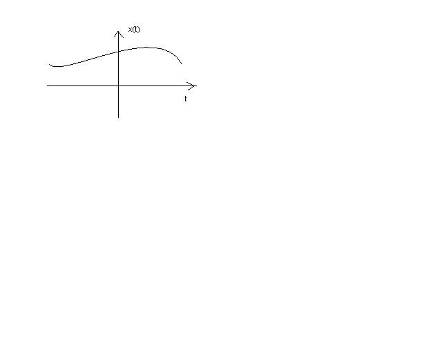
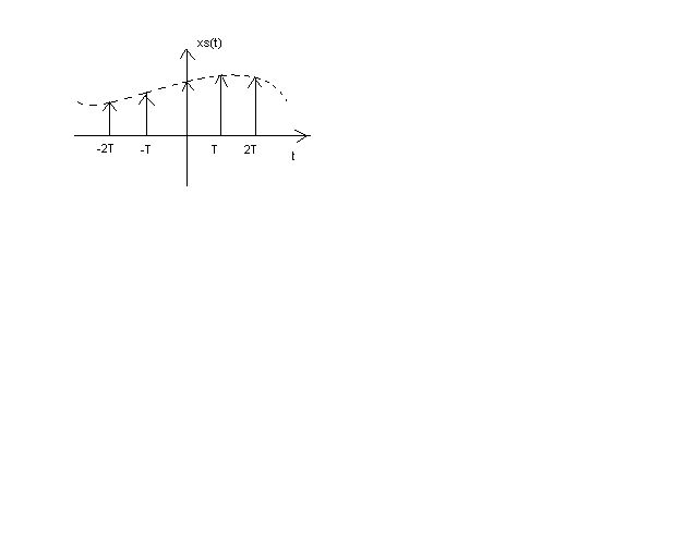
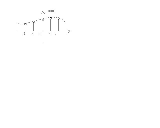
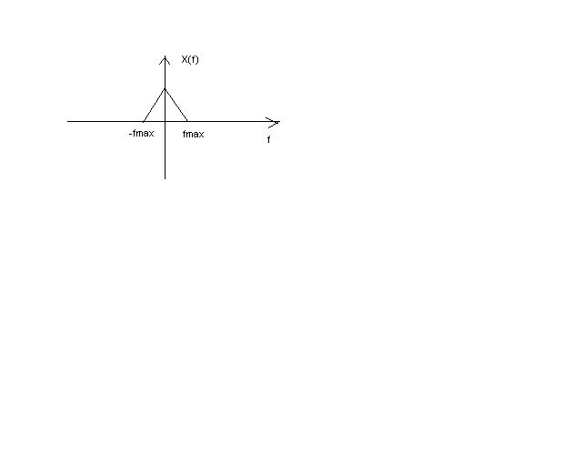
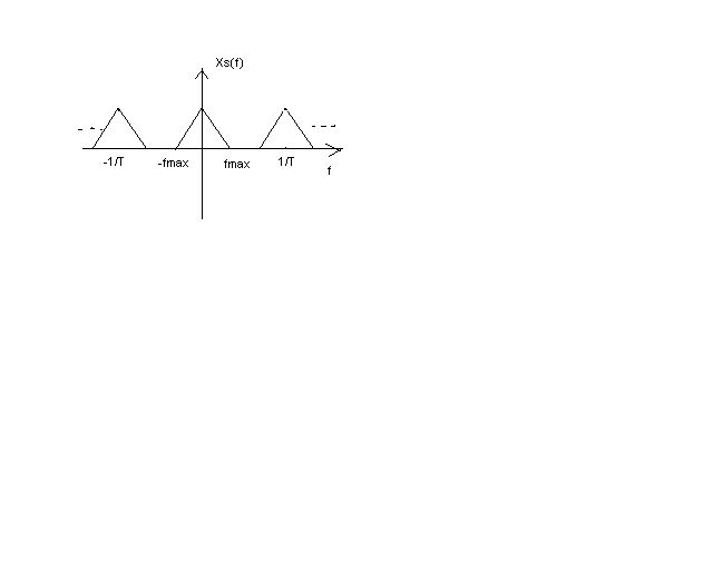
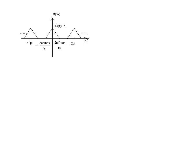Part I: how to convert CT signals to DT signals after sampling. Introduce variables:

                    xc(t)=continuous time signal 
                    xs(t)=signals after sampling
                    x[n]=discrete time signal 

Background: DTFT Xd(ejw)= ∑n=-∞∞ xd[n]e-jwn; -----(1) Sampling, xs(t)=xc(t)pT(t)= ∑n=-∞∞ xc[nTs] δ(t-nTs), where pT(t)= ∑n=-∞∞ δ(t-nTs)

         Xs(f)= CTFT{ ∑n=-∞∞ xc[nTs] δ(t-nTs)}   
               where    1. CTFT{δ(t-nTs)}=∫- ∞∞ δ(t-nTs)e-j2πftdt=e-j2πfnTs
                        2. xc[nTs] is a function of a variable n, and can be rewritten as x[n]
               Therefore, Xs(f)= ∑n=-∞∞ x[n]e-j2πfnTs  OR X(w)= ∑n=-∞∞ x[n]e-j2πwnTs -------(2)  
                          If 2πTs=1, fs=2π, equation (2) can be rewritten as ∑n=-∞∞ x[n]e-jwn,(3)                           

What we can conclude from here is that: if we rescale sampling rate fs as 2π, the sampling signals- a train of impulses can be redrawn to DT signals. The complete expression is X(ejw)=Xs(w/(2πTs))=1/Ts∑n=-∞∞ Xc(w/(2πTs)-n/Ts) We rescaled the original fmax as 2πfmax/fs; also, the amplitude was fs times the initial amplitude from xs(t).