Multivariate Normal Density

Because of the mathematical tractability as well as because of the central limit theorem, Multivariate Normal Density, as known as Gaussian Density, received more attention than other various density functions that have been investigated in pattern recognition.

The general multivariate normal density in d dimensions is:

where

$ \mathbf{x}=[x_1,x_2,\cdots ,x_d]^t $ is a d-component column vector,

$ \mathbf{\mu}=[\mu_1,\mu_2,\cdots ,\mu_d]^t $ is the d-component mean vector,

$ \mathbf{\Sigma}=\begin{bmatrix} \sigma_1^2 & \cdots & \sigma_{1d}^2\\ \vdots & \ddots & \\ \vdots \sigma_{d1}^2 & \cdots & \sigma_d^2 \end{bmatrix} $ is the d-by-d covariance matrix,

$ |\mathbf{\Sigma|} $ is its determinant,

$ \mathbf{\Sigma}^{-1} $ is its inverse.

Each $ p(x_i)\sim N(\mu_i,\sigma_i^2) $, so $ \Sigma $ plays role similar to the role that $ \sigma^2 $ plays in one dimension. Thus, we can find out the relationship among different features (such as $ x_i $ and $ x_j $)through $ \Sigma $:

• $ \sigma_{ij}=0 $, $ x_i $ and $ x_j $ are independent;
• $ \sigma_{ij}>0 $, $ x_i $ and $ x_j $ are positive correlated;
• $ \sigma_{ij}<0 $, $ x_i $ and $ x_j $ are negative correlated.

Discriminant Functions

One of the most useful method to represent pattern classifiers is in terms of a set of discriminant functions $ g_i(\mathbf{x}), i=1,2,...,c $. The classifier is said to assign a feature vector $ \mathbf{x} $ to class $ w_i $ if

Thus, the classification is viewed as process to compute the discriminant functions and select the category corresponding to the largest discriminant. A Bayes classifier is easily represented in this way. In order to simplify the classification process, minimum-error-rate classification is always chosen by taking $ g_i({\mathbf{x}}) $ in natural logarithm format:

Equation (2) can be readily evaluated if the densities $ p(\mathbf{x}|w_i) \sim N(\mathbf{\mu}_i, \mathbf{\Sigma}_i) $. From Equation (1), we have the following discriminant function for multivariate normal density:

we will use Equation (3) to discuss three special classification cases in the next part. To point out that, in next part, two classes two dimension features will be used in the discussion.

Classification for Three Special Cases

Case 1:

$ \mathbf{\Sigma}_i = \sigma^2 \mathbf{I} $

In this case, features $ x_1 $ $ x_2 $ are independent with different means and equal variances. That is,

Thus, $ \mathbf{\Sigma}_i^{-1}=1/\sigma^2 $ and $ \mathbf{\Sigma}_i $ is a constant. So the discriminant function shown in Equation (3) can be simplified to Equation (4):

Expand Equation (4), we obtain

Since $ \mathbf{x}^t \mathbf{x} $ is a constant for all classes, so we can expand Equation (5) continuously,

Since $ \frac{\mathbf{\mu}_i^t}{\sigma^2} $ and $ -\frac{\mathbf{\mu}_i^t \mathbf{\mu}_i}{2 \sigma^2}+\ln P(w_i) $ are constant in $ \mathbf{x} $, so if we let $ w_i=\frac{\mathbf{\mu}_i^t}{\sigma^2} $, $ w_{i0}=-\frac{\mathbf{\mu}_i^t \mathbf{\mu}_i}{2 \sigma^2}+\ln P(w_i) $, we obtain

Thus, from Equation (7), we conclude that in Case I, the classifier is a linear classifier.

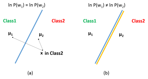
Next, we will explore its geometric interpretation.

Figure 1. Geometric Interpretation of Case 1: (a) two classes have the same prior probability; (b) two classes do not have the same prior probabilities.