(New page: See also: [Fisher Linear Discriminant] In this derivation, we assume the dimension of the space being projected to, k, is k=1. We attempt to find a linear projection (line that passes th...) |
(Removed broken (accidentaly replaced) animation which was not relavant to the discussion any more.) |
||
| (15 intermediate revisions by 3 users not shown) | |||
| Line 1: | Line 1: | ||
| − | See also: [Fisher Linear | + | See also: [[Fisher Linear Discriminant_OldKiwi]] |
In this derivation, we assume the dimension of the space being projected to, k, is k=1. | In this derivation, we assume the dimension of the space being projected to, k, is k=1. | ||
| − | We attempt to find a linear projection (line that passes through the origin) s.t. the projected data can be "best" separated | + | We attempt to find a linear projection (line that passes through the origin) s.t. the projected data can be "best" separated. |
| − | + | Assume <math>y_1,..., y_{d_1}</math> belongs to Class 1 and <math>y_{d_1+1}</math>,..., <math>y_d</math> belongs to Class 2. | |
| − | + | ||
| − | + | ||
| − | + | ||
| − | + | ||
| − | + | ||
| − | + | ||
| − | + | ||
| − | + | ||
| − | + | ||
| − | + | ||
| − | + | ||
| − | + | ||
| − | Assume <math>y_1 | + | |
Consider the sample mean of the projected data for each class | Consider the sample mean of the projected data for each class | ||
| Line 24: | Line 11: | ||
<math>\tilde{m_1} = \frac{1}{d_1} \sum_{i=1}^{d_1} \pi(y_i) = \frac{1}{d_1}\sum_{i=1}^{d_1} \vec{w} \cdot y_i</math>, if <math>||\omega || =1</math> | <math>\tilde{m_1} = \frac{1}{d_1} \sum_{i=1}^{d_1} \pi(y_i) = \frac{1}{d_1}\sum_{i=1}^{d_1} \vec{w} \cdot y_i</math>, if <math>||\omega || =1</math> | ||
| − | + | === Observation 1 === | |
| + | <math>\tilde{m1} = \vec{w} \frac{1}{d_1} \sum_{i=1}^{d_1} y_i</math>, which is the projection of the sample mean for Class 1. | ||
Also, <math>\tilde{m_2} = \frac{1}{d-d_1}\sum_{i=d_1+1}^{d} \vec{w} \cdot y_i = \vec{w} \cdot m_2</math> . | Also, <math>\tilde{m_2} = \frac{1}{d-d_1}\sum_{i=d_1+1}^{d} \vec{w} \cdot y_i = \vec{w} \cdot m_2</math> . | ||
| Line 37: | Line 25: | ||
Define the following cost function, <math>J(\vec{w}) = \frac{|\tilde{m1} - \tilde{m2}|^2}{\tilde{S_1}^2+ \tilde{S_2}^2}</math> . | Define the following cost function, <math>J(\vec{w}) = \frac{|\tilde{m1} - \tilde{m2}|^2}{\tilde{S_1}^2+ \tilde{S_2}^2}</math> . | ||
| − | The above equation is the "[Fisher linear | + | The above equation is the "[[Fisher linear discriminant_OldKiwi]]". |
| − | + | === Observation 2 === | |
| + | Demanding <math>||\tilde{m_1} - \tilde{m_2}||</math> to be maximized would not do, since <math>||\tilde{m_1} - \tilde{m_2}|| = |\vec{w} \cdot m_1 - \vec{w} \cdot m_2 | = | \vec{w} \cdot (m_1 - m_2)| \rightarrow \infty</math> | ||
Need to fix <math>|| \omega || = 1</math> , resulting in a Constrained Optimization Problem. | Need to fix <math>|| \omega || = 1</math> , resulting in a Constrained Optimization Problem. | ||
| − | |||
| − | |||
| − | |||
| − | |||
| − | |||
| − | |||
| − | |||
| − | |||
| − | |||
| − | |||
By dividing by <math>\tilde{S_1}^2 + \tilde{S_2}^2</math> we demand that <math>\vec{w} \cdot (m_1 - m_2)</math> be large in comparison with the scatter. This allows you to bypass the coordinate scale problem because <math>J(\vec{w})</math> is independent of <math>\omega</math>. | By dividing by <math>\tilde{S_1}^2 + \tilde{S_2}^2</math> we demand that <math>\vec{w} \cdot (m_1 - m_2)</math> be large in comparison with the scatter. This allows you to bypass the coordinate scale problem because <math>J(\vec{w})</math> is independent of <math>\omega</math>. | ||
| − | + | <math>|\tilde{m_1} - \tilde{m_2}|^2 = | w(m_1 - m_2)|^2 = |w|^2 | \frac{w}{|w|}(m_1-m_2)|^2</math> | |
| − | + | ||
| − | + | ||
| − | + | ||
| − | + | ||
| − | + | ||
| − | + | ||
| − | + | ||
| − | + | ||
| − | + | ||
Similarly, | Similarly, | ||
| − | | | + | <math>\tilde{S_1}^2 = \sum (\vec{w}(y_i - m_1))^2 = |w|^2 \sum (\frac{w}{|W|} (y_i - m_1))^2</math> |
and, | and, | ||
| − | | | + | <math>\tilde{S_2}^2 = \sum (\vec{w}(y_i - m_1))^2 = |w|^2 \sum (\frac{w}{|W|} (y_i - m_2))^2</math> |
| + | |||
and, | and, | ||
| − | + | <math>J(\vec{w}) = \frac{|m_1-m_2|^2}{S_1^2+S_2^2} =\frac{|w|^2 | \frac{w}{|w|}(m_1-m_2)|^2}{|w|^2(\sum (\frac{w}{|W|} (y_i - m_1))^2 + \sum (\frac{w}{|W|} (y_i - m_2))^2 )} | |
| − | + | </math> is independent of <math>||\omega||</math>. | |
| − | + | ||
| − | + | ||
| − | + | ||
Importance of scatter: | Importance of scatter: | ||
| − | + | [[Image:fld_explanation2_OldKiwi.JPG]] | |
| − | + | ||
| − | + | ||
| − | + | ||
| − | + | ||
| − | + | ||
| − | + | ||
| − | + | ||
| − | + | ||
| − | + | ||
| − | + | ||
| − | + | ||
| − | + | ||
| − | + | ||
| − | + | ||
| − | + | ||
| − | + | ||
| − | + | ||
| − | + | ||
| − | + | ||
| − | + | ||
| − | + | ||
| − | + | ||
| − | + | ||
| − | + | ||
| − | + | ||
| − | + | ||
| − | + | ||
| − | + | ||
| − | + | ||
| − | + | ||
| − | + | ||
| − | + | ||
| − | + | ||
| − | + | ||
| − | + | ||
| − | + | ||
| − | + | ||
| − | + | ||
| − | + | ||
| − | + | ||
| − | + | ||
| − | + | ||
| − | + | If we find <math>\omega</math> which makes <math>Jw</math> large, we are guaranteed that the classes are well-separated. | |
| − | + | ||
| + | [[Image:fld_explanation3a_OldKiwi.jpg]] | ||
| − | + | We can write <math>Jw</math> using matrices: | |
| − | + | <math>J(\vec{w}) = \frac{\vec{w}^{\top}S_B \vec{w}}{\vec{w}^{\top}S_w \vec{w}} | |
| + | </math>, which is called the "[Generalized Rayleigh Quotient]". | ||
| − | ( | + | ([[Lecture 11_OldKiwi]] begins here) |
| − | + | ||
| − | + | Last time we considered <math>J(\vec{w})=\frac {{\vec{w}}^{T}{S}_{B}\vec{w}} {{\vec{w}}^{T}{S}_{W}\vec{w}}</math>, explicit function of <math>\vec{w}</math> | |
| − | + | one can do this because | |
| − | | | + | (numerator of J) = <math>\| \tilde{m_1}-\tilde{m_2} \|^2 = \| w(m_1-m_2) \|^2 = \| (m_1-m_2)^T w \|^2</math> |
| − | + | <math>=w^T (m_1-m_2)(m_1^T-m_2^T)w</math> | |
| − | + | where, <math>(m_1-m_2)(m_1^T-m_2^T) =S_B</math> is 'between class scatter matrix'. | |
| − | + | (denominator of J) = <math>\tilde{s_1}^2 + \tilde{s_2}^2</math> | |
| + | <math>\tilde{s_1}^2 =\displaystyle \sum_{\vec y \; in \; class} (w y_i- \tilde{m_i} )^2 | ||
| + | </math> | ||
| + | <math> = \displaystyle \sum_{\vec{y} \; in \; class} w^T (y_i-m_i)(y_i^T-m_i^T)w</math> | ||
| − | + | <math>w^T \displaystyle \sum_{\vec{y} \; in \; class} (y_i-m_i)(y_i^T-m_i^T)w</math> | |
| − | + | ||
| − | + | ||
| − | + | ||
| − | + | ||
| − | + | where, <math>\displaystyle \sum_{\vec y \; in \; class} (y_i-m_i)(y_i^T-m_i^T) =S_w </math> is 'within class scattter matrix'. | |
Latest revision as of 10:50, 22 April 2008
See also: Fisher Linear Discriminant_OldKiwi
In this derivation, we assume the dimension of the space being projected to, k, is k=1.
We attempt to find a linear projection (line that passes through the origin) s.t. the projected data can be "best" separated.
Assume $ y_1,..., y_{d_1} $ belongs to Class 1 and $ y_{d_1+1} $,..., $ y_d $ belongs to Class 2.
Consider the sample mean of the projected data for each class
$ \tilde{m_1} = \frac{1}{d_1} \sum_{i=1}^{d_1} \pi(y_i) = \frac{1}{d_1}\sum_{i=1}^{d_1} \vec{w} \cdot y_i $, if $ ||\omega || =1 $
Observation 1
$ \tilde{m1} = \vec{w} \frac{1}{d_1} \sum_{i=1}^{d_1} y_i $, which is the projection of the sample mean for Class 1.
Also, $ \tilde{m_2} = \frac{1}{d-d_1}\sum_{i=d_1+1}^{d} \vec{w} \cdot y_i = \vec{w} \cdot m_2 $ .
Consider the scatter projections:
$ \tilde{S_1}^2 = \sum_{i=1}^{d_1} (\vec{w} \cdot y_i - \tilde{m_1})^2 $
$ \tilde{S_2}^2 = \sum_{i=d_1+1}^{d} (\vec{w} \cdot y_i - \tilde{m_2})^2 $
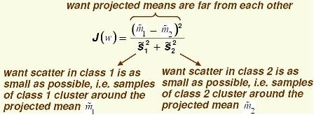
Define the following cost function, $ J(\vec{w}) = \frac{|\tilde{m1} - \tilde{m2}|^2}{\tilde{S_1}^2+ \tilde{S_2}^2} $ .
The above equation is the "Fisher linear discriminant_OldKiwi".
Observation 2
Demanding $ ||\tilde{m_1} - \tilde{m_2}|| $ to be maximized would not do, since $ ||\tilde{m_1} - \tilde{m_2}|| = |\vec{w} \cdot m_1 - \vec{w} \cdot m_2 | = | \vec{w} \cdot (m_1 - m_2)| \rightarrow \infty $
Need to fix $ || \omega || = 1 $ , resulting in a Constrained Optimization Problem.
By dividing by $ \tilde{S_1}^2 + \tilde{S_2}^2 $ we demand that $ \vec{w} \cdot (m_1 - m_2) $ be large in comparison with the scatter. This allows you to bypass the coordinate scale problem because $ J(\vec{w}) $ is independent of $ \omega $.
$ |\tilde{m_1} - \tilde{m_2}|^2 = | w(m_1 - m_2)|^2 = |w|^2 | \frac{w}{|w|}(m_1-m_2)|^2 $
Similarly,
$ \tilde{S_1}^2 = \sum (\vec{w}(y_i - m_1))^2 = |w|^2 \sum (\frac{w}{|W|} (y_i - m_1))^2 $
and,
$ \tilde{S_2}^2 = \sum (\vec{w}(y_i - m_1))^2 = |w|^2 \sum (\frac{w}{|W|} (y_i - m_2))^2 $
and,
$ J(\vec{w}) = \frac{|m_1-m_2|^2}{S_1^2+S_2^2} =\frac{|w|^2 | \frac{w}{|w|}(m_1-m_2)|^2}{|w|^2(\sum (\frac{w}{|W|} (y_i - m_1))^2 + \sum (\frac{w}{|W|} (y_i - m_2))^2 )} $ is independent of $ ||\omega|| $.
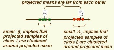
Importance of scatter:
If we find $ \omega $ which makes $ Jw $ large, we are guaranteed that the classes are well-separated.
We can write $ Jw $ using matrices:
$ J(\vec{w}) = \frac{\vec{w}^{\top}S_B \vec{w}}{\vec{w}^{\top}S_w \vec{w}} $, which is called the "[Generalized Rayleigh Quotient]".
(Lecture 11_OldKiwi begins here)
Last time we considered $ J(\vec{w})=\frac {{\vec{w}}^{T}{S}_{B}\vec{w}} {{\vec{w}}^{T}{S}_{W}\vec{w}} $, explicit function of $ \vec{w} $
one can do this because
(numerator of J) = $ \| \tilde{m_1}-\tilde{m_2} \|^2 = \| w(m_1-m_2) \|^2 = \| (m_1-m_2)^T w \|^2 $
$ =w^T (m_1-m_2)(m_1^T-m_2^T)w $
where, $ (m_1-m_2)(m_1^T-m_2^T) =S_B $ is 'between class scatter matrix'.
(denominator of J) = $ \tilde{s_1}^2 + \tilde{s_2}^2 $
$ \tilde{s_1}^2 =\displaystyle \sum_{\vec y \; in \; class} (w y_i- \tilde{m_i} )^2 $
$ = \displaystyle \sum_{\vec{y} \; in \; class} w^T (y_i-m_i)(y_i^T-m_i^T)w $
$ w^T \displaystyle \sum_{\vec{y} \; in \; class} (y_i-m_i)(y_i^T-m_i^T)w $
where, $ \displaystyle \sum_{\vec y \; in \; class} (y_i-m_i)(y_i^T-m_i^T) =S_w $ is 'within class scattter matrix'.


