| Line 8: | Line 8: | ||
A continuous time signal is a function that is continuous, meaning there are no breaks in the signal. For all real values of t you will get a value. <math> f(t), t\subset \mathbb{R} </math> CT signals are ususally represented by using <math>x(t)</math>, having a parentheses and the variable t. | A continuous time signal is a function that is continuous, meaning there are no breaks in the signal. For all real values of t you will get a value. <math> f(t), t\subset \mathbb{R} </math> CT signals are ususally represented by using <math>x(t)</math>, having a parentheses and the variable t. | ||
| + | <gallery> | ||
| + | File:CT_sin_normal.PNG|Graph of sin function in CT | ||
| + | |||
| + | </gallery> | ||
'''Discrete Time (DT) Signals''' | '''Discrete Time (DT) Signals''' | ||
A discrete time signal is a signal whose value is taken at discrete measurements. With a discrete time signal there will be time periods of n where you do not have a value. DT signals are represented using the form <math>x[n]</math>. Discrete signals are approximations of CT signals | A discrete time signal is a signal whose value is taken at discrete measurements. With a discrete time signal there will be time periods of n where you do not have a value. DT signals are represented using the form <math>x[n]</math>. Discrete signals are approximations of CT signals | ||
| + | <gallery> | ||
| + | File:DT_sin_normal.PNG|Graph of sin function in DT | ||
| + | </gallery> | ||
'''Systems''' | '''Systems''' | ||
| Line 30: | Line 37: | ||
! !! CT !!DT | ! !! CT !!DT | ||
|- | |- | ||
| − | ! Time Delay|| <math>x(t) \rightarrow [timeshift] \rightarrow y(t) = x(t-t_0)</math>|| <math>x[n] \rightarrow [timeshift] \rightarrow y[n] = x[n-n_0]</math> | + | ! Time Delay|| <math>x(t) \rightarrow [timeshift] \rightarrow y(t) = x(t-t_0)</math><gallery> |
| + | File:CT_sin_time_shift.PNG| | ||
| + | |||
| + | </gallery>|| <math>x[n] \rightarrow [timeshift] \rightarrow y[n] = x[n-n_0]</math><gallery> | ||
| + | File:DT_sin_time_shift.PNG| | ||
| + | |||
| + | </gallery> | ||
|- | |- | ||
| − | ! Time Reversal|| <math>x(t) \rightarrow [timereversal] \rightarrow y(t) = x(-t)</math>|| <math>x[n] \rightarrow [timereversal] \rightarrow y[n] = x[-n]</math> | + | ! Time Reversal|| <math>x(t) \rightarrow [timereversal] \rightarrow y(t) = x(-t)</math><gallery> |
| + | File:CT_sin_time_reverse.PNG | ||
| + | |||
| + | </gallery>|| <math>x[n] \rightarrow [timereversal] \rightarrow y[n] = x[-n]</math><gallery> | ||
| + | File:DT_sin_time_reversal.PNG | ||
| + | |||
| + | </gallery> | ||
|- | |- | ||
| − | ! Time Scaling|| <math>x(t) \rightarrow [timescaling] \rightarrow y(t) = x(at)</math>|| <math>x[n] \rightarrow [timeshift] \rightarrow y[n] = x[an]</math> | + | ! Time Scaling|| <math>x(t) \rightarrow [timescaling] \rightarrow y(t) = x(at)</math><gallery> |
| + | File:CT_sin_time_scaling.PNG | ||
| + | |||
| + | </gallery>|| <math>x[n] \rightarrow [timeshift] \rightarrow y[n] = x[an]</math><gallery> | ||
| + | File:DT_sin_time_scaling.PNG | ||
| + | |||
| + | </gallery> | ||
|} | |} | ||
Revision as of 16:57, 2 December 2018
The aim of this is to show the student the difference between Continuous and Discrete signals and systems, and how to identify them.
Signal
A signal is a function, so when we say a continuous time signal or a discrete time signal we really mean continuous time functions and discrete time functions.
Continuous Time (CT) Signals
A continuous time signal is a function that is continuous, meaning there are no breaks in the signal. For all real values of t you will get a value. $ f(t), t\subset \mathbb{R} $ CT signals are ususally represented by using $ x(t) $, having a parentheses and the variable t.
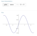
Graph of sin function in CT

Discrete Time (DT) Signals
A discrete time signal is a signal whose value is taken at discrete measurements. With a discrete time signal there will be time periods of n where you do not have a value. DT signals are represented using the form $ x[n] $. Discrete signals are approximations of CT signals
- DT sin normal.PNG
Graph of sin function in DT
Systems
A system transforms one signal into a different signal
Continuous Time (CT) System
A continuous time system can be likened to an analog to analog system. It takes in an analog(CT) signal and outputs ad different analog signal
Discrete Time (DT) System
A discrete time system can be likened to a discrete to discrete system. It takes in DT signal and outputs a different DT signal. Recordings are a good example for DT systems because when you record a sound you are taking samples at very close together time points to digitally recreate the sound
Basic System Types
| CT | DT | |
|---|---|---|
| Time Delay | $ x(t) \rightarrow [timeshift] \rightarrow y(t) = x(t-t_0) $ |
$ x[n] \rightarrow [timeshift] \rightarrow y[n] = x[n-n_0] $ |
| Time Reversal | $ x(t) \rightarrow [timereversal] \rightarrow y(t) = x(-t) $ |
$ x[n] \rightarrow [timereversal] \rightarrow y[n] = x[-n] $ |
| Time Scaling | $ x(t) \rightarrow [timescaling] \rightarrow y(t) = x(at) $ |
$ x[n] \rightarrow [timeshift] \rightarrow y[n] = x[an] $ |


Examples of CT and DT systems
| CT System | DT System |
|---|---|
| $ noise\, from\, lips\, \rightarrow [trumpet]\rightarrow trumpet\, noise $ | $ recorded\, noise \rightarrow [software\, to \, sound\, like\, trumpet] \rightarrow trumpet\, sound $ |
| $ visual \, of \, cat \rightarrow [ hand\, drawn \, cat] \rightarrow picture\, of \, cat $ | $ visual\, of\, cat\, \rightarrow [camera\, picture] \rightarrow picture\, of\, cat $ |
| $ sound \rightarrow [analog\, microphone] \rightarrow louder\, sound $ | $ sound \rightarrow [digital\, microphone] \rightarrow louder\, sound $ |