(→Experiments with poorly correlated data) |
|||
| Line 14: | Line 14: | ||
=== Experiments with poorly correlated data === | === Experiments with poorly correlated data === | ||
| − | [[Image: | + | [[Image:Lcd_OldKiwi.jpg|none|500px|left|thumb|Figure 3]] |
| − | [[Image: | + | [[Image:Lca_OldKiwi.jpg|none|500px|left|thumb|Figure 4]] |
| + | |||
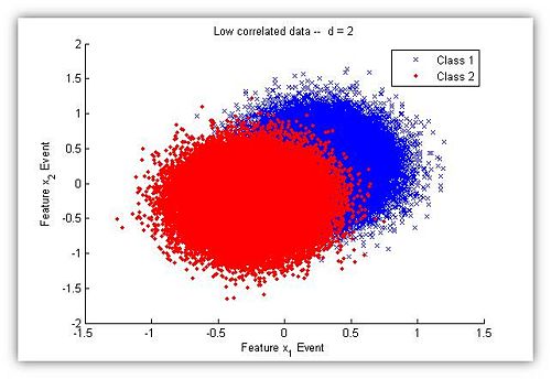
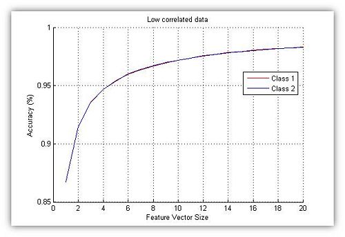
| + | In this experiment, we expected the accuracy to converge to one. There are a low correlation between features in class 1 and class2. Therefore, with each extra feature we can be sure that we are doing a better categorization of the samples. Our expectations were achieved as shown in Figure 4. | ||
=== Experiments with highly/poorly correlated data=== | === Experiments with highly/poorly correlated data=== | ||
Revision as of 22:44, 8 March 2008
Maybe you will think that the categorization accuracy of Bayes system goes down as the number of features goes up. The fact is that as we increase the size of the feature vector we have more elements to describe and categorize a class. Therefore, more features should not be bad. The issue is that if we add features with high correlation between classes, the information provided by those features is almost useless. The classes at those features are not separable, so we cannot make a good decision based on highly correlated features. Consequently, when we are characterizing classes by their features, we need to select features that have poor correlation between the classes. Then, the information in the feature vector is meaningful for our categorization. The more meaningful features we have the more accurate the system will be.
The setup for the experiment should be the following. We only have two classes, Class 1 and Class 2. You can test your algorithms for different priori probabilities for Class 1 and Class 2. However if you are working with synthetic data, it is better to have equal priori probabilities to analyze the data. First, generate Gaussian data to train and test the system. We generated N = 105 samples. Also, the variance for each feature was the same and the mean of each class feature changed depending on the hypothesis we wanted to test. Then for each data set, compute the probability model parameters—mean and covariance matrix. Consequently, use Bayes decision formula to categorize the data. Kept track of the accuracy of the system for each feature vector size. The size of our feature vector was in the range of 1 to 20 features. Our measure of accuracy was the number of samples classified correctly divided by the total number of samples for the class (N = 105).
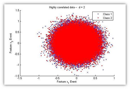
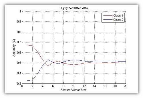
As you can see in Figure 1 the classes are highly correlated. In Figure 2, you can observe that as we increase the size of the feature vector the accuracy converges close to 50%. The brute force approach is to classify the sample in either class, for an expected accuracy of 50%. Consequently, data that is highly correlated, increasing the feature vector size does not help. We need to recall that the accuracy results directly depend on the data we are analyzing. Therefore, we can expect the accuracy to goes up or down for different data sets. Although, we can conclude that the accuracy will be close to 50% for very similar data distributions.
In this experiment, we expected the accuracy to converge to one. There are a low correlation between features in class 1 and class2. Therefore, with each extra feature we can be sure that we are doing a better categorization of the samples. Our expectations were achieved as shown in Figure 4.


