| Line 37: | Line 37: | ||
[[Image:Upsampling_diag.png]] | [[Image:Upsampling_diag.png]] | ||
| − | The first block is the up-sample by <math> N </math> operator, where <math> N\in \mathbb{N} </math>. This inserts <math> N-1 </math> zeros between each point in the time domain. In the DTFT domain, this has the effect of scaling the omega axis by <math> 1/N </math>. This yields the following plot <math> | + | The first block is the up-sample by <math> N </math> operator, where <math> N\in \mathbb{N} </math>. This inserts <math> N-1 </math> zeros between each point in the time domain. In the DTFT domain, this has the effect of scaling the omega axis by <math> 1/N </math>. This yields the following plot <math> U(\omega) </math>. |
[[Image:U_w_plot.png]] | [[Image:U_w_plot.png]] | ||
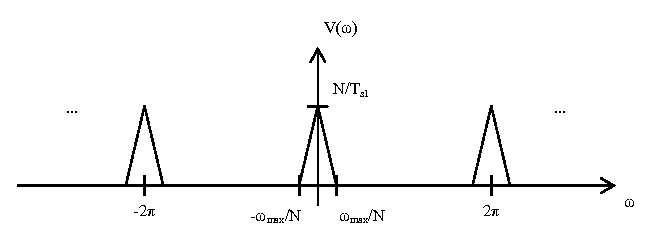
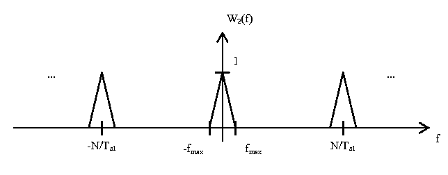
| − | a | + | The next block is a discrete-time low pass filter with gain <math> N </math> and cutoff frequency <math> f_c = \frac{\pi}{N} </math>. This removes all extra DTFT components not centered around <math> 2\pi k, \forall k \in \mathbb{Z} </math>, and scales the magnitude axis by N. This yields the following plot <math> V(\omega) </math>: |
[[Image:V_w_plot.png]] | [[Image:V_w_plot.png]] | ||
| + | |||
| + | a | ||
| + | |||
[[Image:W2_f_plot.png]] | [[Image:W2_f_plot.png]] | ||
== How Analog Filter Design is Affected == | == How Analog Filter Design is Affected == | ||
Revision as of 18:40, 22 September 2009
Contents
Introduction
With microprocessors becoming ever increasingly faster, smaller, and cheaper, it is preferable to use digital signal processing as a way to compensate for distortions caused by analog circuitry. One area that this can be applied is in signal reconstruction, where a low pass analog filter is used on the output of a digital-to-analog converter to attenuate unwanted frequency components above the Nyquist frequency.
The problem with analog low pass filters is that higher the order, the more resistors, capacitors, and op-amps are required in its construction. More circuit components means more circuit board space, which is a precious commodity with today's hand-held devices.
Here, it will be explained how up-sampling can be used to relax requirements on analog low pass filter design while decreasing signal distortion.
A Representative DT Signal
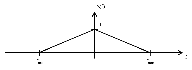
For this discussion, a representative signal $ x(t) $ will be used to demonstrate the process of signal reconstruction. We will look at the signal in the frequency domain, as shown in the plot below:
As seen in the plot, the signal $ X(f) $ has a triangular shape and is band-limited by $ f_{max} $. By the Nyquist-Shannon Sampling Theorem, the sampling frequency $ f_{s1} $ must be greater than $ 2f_{max} $. For this discussion, assume $ f_{s1} $ is just slightly greater than $ 2f_{max} $.
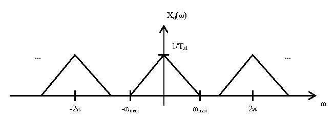
Now, we are going to sample $ x(t) $ with an impulse train with period $ T_{s1} = 1/f_{s1} $ and convert to a discrete time signal. This has the affect of scaling the magnitude axis of $ X(f) $ by $ 1/T_{s1} $ and the frequency axis by $ 2\pi T_{s1} $, and then repeating the result every $ \omega = 2\pi $. This yields the following plot $ X_d(\omega) $:
Without Up-sampling
First, consider the process of signal reconstruction without up-sampling. The following diagram shows the process:
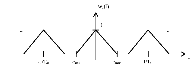
The first block is a digital-to-analog converter. This converts the discrete time signal to a continuous time signal. This has the effect of scaling the magnitude axis by $ T_{s1} $ and the omega axis by $ \frac{1}{2\pi T_{s1}} $. This yields the following plot $ W_1(f) $:
The next step is to use an analog low pass filter to remove all frequency components above $ \frac{1}{2T_{s1}} $. The important note to take from $ W_1(f) $ is that the frequency gap for which the analog filter has to transition from low attenuation to high attenuation is $ \frac{1}{T_{s1}} - 2f_{max} $.
With Up-sampling
Now, consider the process of signal reconstruction with up-sampling. The following diagram shows the process:
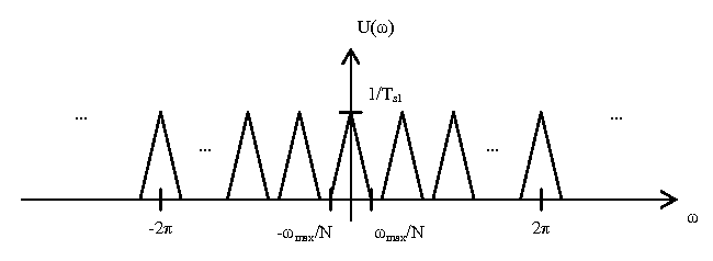
The first block is the up-sample by $ N $ operator, where $ N\in \mathbb{N} $. This inserts $ N-1 $ zeros between each point in the time domain. In the DTFT domain, this has the effect of scaling the omega axis by $ 1/N $. This yields the following plot $ U(\omega) $.
The next block is a discrete-time low pass filter with gain $ N $ and cutoff frequency $ f_c = \frac{\pi}{N} $. This removes all extra DTFT components not centered around $ 2\pi k, \forall k \in \mathbb{Z} $, and scales the magnitude axis by N. This yields the following plot $ V(\omega) $:
a

