Walther MA271 Fall2020 topic25 - Rhea

Maximum Principle in Analysis

Author: Alex Beers

Table of Contents

1. Introduction and Overview
2. What is a Partial Differential Equation
3. The Maximum Principle and Parabolic PDEs
4. Minimums
5. Applications

Introduction and Overview

The Maximum Principle in analysis describes where maximum values can be found for functions described by parabolic and elliptic partial differential equations. These partial differential equations (PDEs) will be explained later on, but for now they can be thought of as equations that describe how a function’s value at any point changes, as opposed to what the value actually is. The Maximum Principle states that the maximum value for a function described by a PDE occurs at the edge of the domain. There is one exception, that being the function having a constant value, in which the maximum value would be everywhere.

This principle can also be applied to finding minimums, which makes it a practical tool in mathematics for finding the max or min of a function described by a PDE, as only the boundary of the domain has to be checked. It also has many applications in physics and engineering, one of the most common of which has to do with quantities that tend to disperse or approach some equilibrium over time, such as temperature, concentration, or pressure, among many others. These real world applications also have nice implications for learners, in that the principle has many intuitive properties.

What is a Partial Differential Equation

Partial differential equations describe the rates of change of functions with multiple independent variables. They are used because it is often easier to describe how a value is changing at some point, rather than what the value actually is. For the best possible introduction to PDEs, I would check out the 17 minute video by 3 Blue 1 Brown on the subject. It is the first link in the references below and provides wonderful graphical intuition via animations, which simply cannot be described here. That said, an explanation is provided here as well.

To first understand Partial Differential Equations, we have to understand Partial Derivatives. Partial derivatives are an extension of normal derivatives (one independent variable) to multiples independent variables. The trick is that we consider all of the independent variables constant except for one. An example is shown below for a function with independent variables x and y.

The partial derivative with respect to x (called partial x) is the rate of change of the function as we walk along a line parallel to the x axis. If y = 0, the function is always 5, so it makes sense that partial x is always 0. If y is positive, the function positively increases as we walk parallel to the y axis, as shown by the partial equation. Higher order partials can be taken in the same manner.

Partials derivatives are the language used to describe PDEs. A simple example PDE is shown below

This PDE, while not that exciting, is a good warm up. It says that partial x is equal to x at all points. If the slope with respect to x is always x, the function described by the PDE is similiar to $ \frac{1}{2}x^2 $.

The Maximum Principle and Parabolic PDEs

Parabolic PDEs, for our purposes, will be considered to deal with time and and tend towards some equilibrium. This is a big generalization, but will work for explaining the basics of the Maximum Principle. More information can be found in the refrences below about parabolic PDEs. These equations describe a range of time dependent processes such as heat dispersion, diffusion of particles, and even economic models. All of these processes can be described by what is called “the heat equation” which was created to describes how heat flows throughout an object over time. We will focus on the heat equation here, as it leads to an incredibly intuitive explanation of the Maximum Principle.

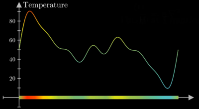
Suppose a rod is heated up and has a temperature distribution as shown below in Fig. 1, where the graph represents the temperature at any point along the rod.

Intuitively, which parts along the rod would cool down the fastest? It would seem that hot portions surrounded by cold neighbors would cool down the fastest, and cold portions with hot neighbors would warm up the fastest. In addition, a portion whose neighbor is say, 10 degrees colder on one side, and 10 degrees warmer on the other side would stay the same temperature — the average of the two neighbors. Looking back at Fig. 1, we may begin to recognize a pattern — portions with high concavity experience the highest temperature change over time. Since concavity can be described by the second derivative of position here, we can say

where $ \alpha $ is a proportionality constant, and can be expanded to

to describe objects in more than one dimension. This is the heat equation, and an example of a parabolic PDE. Once again, the higher the second partial derivative of temperature with respect to any axis (concavity) the higher the rate of change of temperature at any given moment in time.

With this, we have a mathematical model for an object whose peaks are eroded over time, and whose valleys are filled in. It then makes sense that the largest temperature — the largest peak — can only be present at the beginning. By definition, all of the values around the maximum are smaller, and thus concavity will be negative. This will lead to the temperature of that point cooling down immediately after the beginning, moving towards the average. It then makes sense intuitively that the maximum temperature recorded can occur anywhere on the spatial domain, as long as it is at the very beginning.

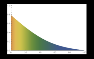
The heat equation, and thus parabolic PDEs, can be extended to describe objects that have points in space on their boundary held at a constant temperature. This has the effect of removing or adding heat from the entire system. The equilibrium state, however, still makes sense intuitively. Temperatures of points in space will tend towards the line of average connecting the two, as shown in Fig. 2 below. One can imagine a scenario where all points on a rod are initially at 0 degrees, but the endpoints are kept at 100 degrees and 0 degrees respectively. The maximum temperature would always be found at the 100 degree point, and all of the middle points would fall somewhere in between.