| Line 5: | Line 5: | ||
<font size="2">(partially based on Prof. [https://engineering.purdue.edu/~mboutin/ Mireille Boutin's] ECE [[ECE662|662]] lecture) </font> | <font size="2">(partially based on Prof. [https://engineering.purdue.edu/~mboutin/ Mireille Boutin's] ECE [[ECE662|662]] lecture) </font> | ||
</center> | </center> | ||
| − | [[Media:MATLAB_code_PCA.zip|MATLAB code]] | + | [[Media:MATLAB_code_PCA.zip|MATLAB code]] |
| + | |||
---- | ---- | ||
| + | |||
---- | ---- | ||
| + | |||
= What will you learn from this slecture? = | = What will you learn from this slecture? = | ||
| − | *A toy example | + | *A toy example to illustrate the idea of PCA |
| − | *The mathematical reasoning behind | + | *The mathematical reasoning behind PCA |
| − | *The strength and limitation of PCA and | + | *A working example using PCA with Bayes rule in classification |
| + | *The strength and limitation of PCA and a brief introuction on various extensions of PCA | ||
<br> | <br> | ||
| Line 20: | Line 24: | ||
== Prerequisite == | == Prerequisite == | ||
| − | This tutorial only requires a working knowledge of basic linear algebra. If you are familiar with standard deviation, covariance and eigen decompostion, then you are fine. | + | This tutorial only requires a working knowledge of basic linear algebra. If you are familiar with standard deviation, covariance and eigen decompostion, then you are fine. Otherwise, Gilbert Strang's great book<sup>[1]</sup> is of great help.<br> |
---- | ---- | ||
| Line 26: | Line 30: | ||
== Introduction == | == Introduction == | ||
| − | Principle Component Analysis (PCA) is a statistical method that uses orthonormal transformations to convert the observed correlated data into a set of linearly uncorrelated data, which are the so-called principle components. PCA has found numerous application fields like face recognition, dimension reduction, factor analysis and image compression, etc. Generally speaking, it's a common technique that can find certain patterns in high-dimension data, and | + | Principle Component Analysis (PCA) is a statistical method that uses orthonormal transformations to convert the observed correlated data into a set of linearly uncorrelated data, which are the so-called principle components. PCA has found numerous application fields like face recognition, dimension reduction, factor analysis and image compression, etc. Generally speaking, it's a common technique that can find certain patterns in high-dimension data, and by considering the most significant patterns only, it can reduce the computation efforts dramatically. When dealing with high-dimension data, it's always not easy for us to visualize the distribution of data, and thus it's very hard to find certain patterns from data which could potentially lead to a better design of classifier. PCA could help us in this case, to find the significant patterns. |
This tutorial is divided into four sections | This tutorial is divided into four sections | ||
| − | #A toy example | + | #A toy example of PCA |
| − | #Mathematical derivation | + | #Mathematical derivation of PCA |
#Use PCA with Bayes rule in classification | #Use PCA with Bayes rule in classification | ||
#Discussion | #Discussion | ||
| Line 37: | Line 41: | ||
== A toy example == | == A toy example == | ||
| − | In this section, I will just use PCA on a simple data set to help you gain some intuition of PCA, the question of "why does it work" is not answered in this section, we just focus on "how to make it work". Then after you get | + | In this section, I will just use PCA on a simple data set to help you gain some intuition of PCA, the question of "why does it work" is not answered in this section, we just focus on "how to make it work". Then after you get hopefully some idea of PCA from this toy example, we will provide the mathematical derivation to explain why it works like this. |
There are basically 6 steps in the procedure of using PCA, they are 1) Construct the data set, 2) Subtract the mean, 3) Calculate the covariance matrix, 4) Get eigenvalue decomposition of covariance matrix, 5) Choose the significant principle components, 6) Get the transformed data. Now we will go through all of them in detail. | There are basically 6 steps in the procedure of using PCA, they are 1) Construct the data set, 2) Subtract the mean, 3) Calculate the covariance matrix, 4) Get eigenvalue decomposition of covariance matrix, 5) Choose the significant principle components, 6) Get the transformed data. Now we will go through all of them in detail. | ||
| Line 43: | Line 47: | ||
=== <font size="2">'''Step 1: Construct the data set'''</font> === | === <font size="2">'''Step 1: Construct the data set'''</font> === | ||
| − | The data set I choose is only two dimension, because it's | + | The data set I choose is only of two dimension, because it's easy for visualization. The original data set is shown below in Figure1. This is only a made-up data, there are 19 observations. As we can easily find, there is a positive correlation between data in the two dimensions. |
| − | + | <center>[[Image:New Original data.jpg|center]]</center> <center>Figure 1. Original data set, data dimension is 2 with 19 observations </center> | |
| − | <center>[[Image:New Original data.jpg|center]]</center> | + | <font size="2">'''Step 2: Subtract the mean'''</font><br> PCA requires the data set to have zero mean in each of the dimensions. Thus we have to subtract the mean, which is the sample average, in each dimension. The sample average for the data in dimension 1 is 5.5 and for data in dimension 2 is 5.7283. Then for the data in each dimension, we subtract the corresponding mean from the original data, the shifted data is shown in Figure 2. From now on, we will just refer the "shifted data" as "original data", unless stated explicitly. |
| − | + | <center>[[Image:New Shifted data.jpg|center]]</center> <center>Figure 2. Shifted data set after subtracting the sample average from the data in each dimension </center> | |
| − | <center>Figure 1. Original data set, data dimension is 2 | + | |
| − | + | ||
| − | <font size="2">'''Step 2: Subtract the mean'''</font><br> PCA requires the data set to have zero mean in each of the dimensions | + | |
| − | + | ||
| − | <center>[[Image:New Shifted data.jpg|center]]</center> | + | |
| − | + | ||
| − | <center>Figure 2. Shifted data set | + | |
| − | + | ||
'''Step 3: Calculate the covariance matrix''' | '''Step 3: Calculate the covariance matrix''' | ||
| Line 61: | Line 57: | ||
, | , | ||
| − | N is the number of observations, notice that this is an unbiased estimate of the true covariance estimate, the derivation of this formula is beyond the scope of this tutorial. | + | N is the number of observations, notice that this is an unbiased estimate of the true covariance estimate, the derivation of this formula is beyond the scope of this tutorial. Using the above formula, we get the covariance |
<center><math> Cov = \begin{bmatrix} 7.9167 & 8.2813 \\[0.3em] 8.2813 & 9.1552 \end{bmatrix}</math></center> | <center><math> Cov = \begin{bmatrix} 7.9167 & 8.2813 \\[0.3em] 8.2813 & 9.1552 \end{bmatrix}</math></center> | ||
, | , | ||
| − | notice that the off-diagonal elements are positive, this implies a positive correlation between the data in the two dimensions. | + | notice that the off-diagonal elements are positive, this implies a positive correlation between the data in the two dimensions, i.e., they will increase together. |
'''Step 4: Get eigenvalue decomposition of the covariance matrix''' | '''Step 4: Get eigenvalue decomposition of the covariance matrix''' | ||
| Line 72: | Line 68: | ||
<center><math> Eigenvector = \begin{bmatrix} -0.7330 & 0.6802 \\[0.3em] 0.6802 & 0.7330 \end{bmatrix}, \quad | <center><math> Eigenvector = \begin{bmatrix} -0.7330 & 0.6802 \\[0.3em] 0.6802 & 0.7330 \end{bmatrix}, \quad | ||
Eigenvalue = \begin{bmatrix} 0.2315 \\[0.3em] 16.8404 \end{bmatrix}</math> </center> | Eigenvalue = \begin{bmatrix} 0.2315 \\[0.3em] 16.8404 \end{bmatrix}</math> </center> | ||
| − | Notice that both eigen vectors are unitary vector, i.e. their length is 1. Now we plot the eigenvector together with data set in Figure 3. The red line indicates the direction | + | Notice that both eigen vectors are unitary vector, i.e. their length is 1. Now we plot the eigenvector together with data set in Figure 3. The red line indicates the direction of the eigenvector for the smaller eigenvalue, and the blue line indicates the direction of the eigenvector for the larger eigenvalue. First notice is that the two eigenvectors are perpendicular to each other , as expected. More importantly, the direction of the eignevector shows a significant pattern in the data set. It's easy to find out that the blue line goes through all the data points and it is a very good fit to the data. While the red line hardly reveals any trend of the distribution of data. To illustrate the phenomenon better, we also draw the line of best fit using least square regression in magenta. As we can see, the blue line and magenta line are very close to each other, both of them are a good fit for the data set. |
| − | + | <center>[[Image:Eigenvector.jpg|center]] </center> <center>Figure 3. Illustration of original data set, eigenvector directions and the best-fit line using least square </center> | |
| − | <center>[[Image:Eigenvector.jpg|center]] </center> | + | |
| − | + | ||
| − | <center>Figure 3. | + | |
| − | + | ||
'''Step 5: Choose the significant principle components''' | '''Step 5: Choose the significant principle components''' | ||
| − | Now we come to the stage of choosing significant principle components. The originical data is in 2 dimension, and now we want to reduce it into 1 dimension. Notice that a 1 dimensional data will form a line in 2D space. So reduce the data from 2D to 1D could also be interpreted as projecting | + | Now we come to the stage of choosing significant principle components. The originical data is in 2 dimension, and now we want to reduce it into 1 dimension. Notice that a 1 dimensional data will form a line in 2D space. So reduce the data from 2D to 1D could also be interpreted as projecting the original data sets onto a line, and this line could preserve the most amount of information of the original 2D data set. Notice that we can't preserve all the information after projection, we can only compress the original information and represent it in a lower dimension, which could be still useful in some sense. Here we define the sum of square distances between the original data set and the projected data set as the error of the projection, or as a measure of loss of information. Since now from the eigen decomposition of the covariance matrix, we get two vectors which represent two lines, we will just blindly follow these lines and project our original data set onto them, then compare the loss of information after the projection. Here we will define the direction which is decided by the eigenvector as "principle direction". |
| − | + | ||
| − | + | ||
| − | + | ||
| − | + | ||
| − | + | ||
| − | + | ||
| − | + | ||
| − | + | ||
| − | + | ||
| − | + | ||
| − | + | ||
| − | + | ||
| − | + | ||
| − | + | ||
| − | + | ||
| − | + | ||
| − | + | ||
| − | + | ||
| − | + | ||
| − | + | Figure 4 and Figure 5 show the projection for these two principle directions, respectively. In each figure, the black dots are the original data set, the black line shows the direction of the eigenvector, the blue dots are the points which are projections from the original data onto the principle direction. And the red line indicates the distance between the original data and the projected data, hence the error of the projection. We would like to find a way of projection which could minimize the total error. Obviously, from the figure we know that the projection onto the direction which is specified by the eigenvector of the larger eigenvalue is favored. In fact, the sum of errors of projection in Figure 4 is 7.17 and the sum of errors of projection in Figure 5 is 64.6. Without doubt, if we want to project the original data from 2D to 1D, we will choose the eigenvector or the larger eigenvalue as projection axis. Now we get an intuition that the eigenvectors which correspond to larger eigenvalues could provide more significant patterns of the data, thus could be chosen to generate significant principle components. | |
| − | <center>Figure | + | In general, the procedure to choose the significant principle components contain the following steps: 1) get the eigendecomposition of the covariance matrix, 2) sort the eigenvalues in decreasing order, and swap the eigenvectors correspondly, 3) choose the largest p eigenvalues and the corresponding eigenvectors to serve as a basis for the new space which the reduced or compressed data lie in. The value of p is chosen based on a user-definied criterion, like the sum of energy should be at least 90% of the original energy, or the sum or error could not exceed a threshold, 4) stack these eigenvectors to form a feature vector, which serves as the basis for the reduced space. |
| + | <center><math> FeatureVector = \begin{bmatrix} EigenVec 1 & EigenVec 2 & ... & EigenVec P\end{bmatrix} </math> </center> <center>[[Image:Projection large evalue.jpg|center]] </center> <center>Figure 4: Projection onto the eigenvector direction which corresponds to the '''large '''eigenvalue.</center> <center>[[Image:Projection small evalue.jpg|center]] </center> <center>Figure 5: Projection onto the eigenvector direction which corresponds to the '''small '''eigenvalue </center> | ||
| + | <br> '''Step 6: Get the transformed data''' | ||
| + | Notice that after the projection, the projected data are still in 2D. And we have not really compressed the data yet. To accomplish that, we need to rotate the line and put the line in 1D, so that the reduced data is represented by only one variable. Actually the projection and rotation could be combined into one step only, that is to multiply the original data by the feature vector. The formula is | ||
| + | <center><span class="texhtml">''R''''e''''d''''u''''c''''e''''d''''D''''a''''t''''a'' = ''O''''r''''i''''g''''i''''n''''a''''l''''D''''a''''t''''a'''''<b> * ''F'''</b>''e''''a''''t''''u''''r''''e''''V''''e''''c''''o''''t''''o''''r''</span></center> | ||
| + | <br> Based on the organization of the original data, we might need to transpose the OriginalData matrix, just to make sure that the matrix multiplication could enjoy the right size of each matrix. In Figure 6, the reduced data is shown. It's only a line (1D data) shown in 2D. As we can see, this is the rotation of the projection in Figure 4. To get the original data back, we notice that the featurevector matrix is orthonorma, thus we have the formula, | ||
| + | <center><span class="texhtml">''O''''r''''i''''g''''i''''n''''a''''l''''D''''a''''t''''a'''''<b> = ''R'''</b>''e''''d''''u''''c''''e''''d''''D''''a''''t''''a'''''<b> * ''F'''</b>''e''''a''''t''''u''''r''''e''''V''''e''''c''''t''''o''''r'''''<b><sup>''T''</sup></b></span></center> | ||
| + | '''<br>''' | ||
| + | <center>[[Image:PCA reduced data.jpg|center]] </center> <center>Figure 6: The PCA reduced data in 1D.</center> | ||
<br> | <br> | ||
| − | Throughout this section, I illustrated a toy example of PCA to give you a general idea and hopefully some intuition of how PCA works. After we use PCA to reduce the data from original dimension to a lower dimension, we could use this compressed data set as an efficient representation of the original data, | + | Throughout this section, I illustrated a toy example of PCA to give you a general idea and hopefully some intuition of how PCA works. After we use PCA to reduce the data from original dimension to a lower dimension, we could use this compressed data set as an efficient representation of the original data, and further could make some decision making processing based on this reduced data set to save computational resources. In the next section we will focus more on the mathematical theories behind PCA, trying to explain why it works. |
== Mathematical derivation == | == Mathematical derivation == | ||
| − | In this chapter we will explore the mathematical theories behind PCA to understand why it works. PCA can be defined as the orthogonal projection of the data onto a lower dimensional linear space, known as the ''principle subspace'', such that the variance of the projected data is maximized<sup>[3]</sup> | + | In this chapter we will explore the mathematical theories behind PCA to understand why it works. PCA can be defined as the orthogonal projection of the data onto a lower dimensional linear space, known as the ''principle subspace'', such that the variance of the projected data is maximized<sup>[3]</sup> (other definition and derivation of PCA could be found in [4]). Following this idea of maximizing variance, let's derive the formula for PCA. |
| − | The dataset contains observations <span class="texhtml">''x''<sub>''n''</sub></span>, where <span class="texhtml">''n'' = 1,...,''N''</span>, and <span class="texhtml">''x''<sub>''n''</sub></span> is a variable with dimension <span class="texhtml">''M''</span>. Our goal is to project the data onto a subspace which has dimension <span class="texhtml">''P'' < ''M''</span> while maximizing the variance of the projected data. For now we will assume that <span class="texhtml">''P''</span> is given, i.e. the dimension of the subspace | + | The dataset contains observations <span class="texhtml">''x''<sub>''n''</sub></span>, where <span class="texhtml">''n'' = 1,...,''N''</span>, and <span class="texhtml">''x''<sub>''n''</sub></span> is a variable with dimension <span class="texhtml">''M''</span>. Our goal is to project the data onto a subspace which has dimension <span class="texhtml">''P'' < ''M''</span> while maximizing the variance of the projected data. For now we will assume that <span class="texhtml">''P''</span> is given, i.e. we are already given the dimension of the subspace. |
| − | | + | First, let's consider the projection onto a one-dimensional space (<span class="texhtml">''P'' = 1</span>). To define the direction of this subspace, we use a <span class="texhtml">''M''</span>-dimensional unit vector <span class="texhtml">''u''<sub>1</sub></span> so that <math> u_1^Tu_1 = 1 </math> , this is for convenience and without loss of generality. Notice that here only the direction defined by <span class="texhtml">''u''<sub>1</sub></span> is of interest to us, the magnitude of <span class="texhtml">''u''<sub>1</sub></span> is not critical. After we define the direction of the subspace, each data point <span class="texhtml">''x''<sub>''n''</sub></span> is projected onto this subspace, and we get a scalar <math> u_1^Tx_n </math> as the result of each projection. The mean of the projected data is <math>u_1^T\bar{x} </math> , where <math> \bar{x} </math> is the sample mean of the original data set given by |
<center><math> \bar{x} = \frac{1}{N}\sum_{n=1}^{N}x_n </math> </center> | <center><math> \bar{x} = \frac{1}{N}\sum_{n=1}^{N}x_n </math> </center> | ||
and the variance of the projected data which lies in the subspace is given by | and the variance of the projected data which lies in the subspace is given by | ||
| Line 127: | Line 108: | ||
we get | we get | ||
<center><math>Su_1=\lambda_1u_1 \implies u_1^TSu_1 = \lambda_1</math></center> | <center><math>Su_1=\lambda_1u_1 \implies u_1^TSu_1 = \lambda_1</math></center> | ||
| − | from the above equation we got the conclusion that 1) <span class="texhtml">''u''<sub>1</sub></span> must be an eigenvector of <span class="texhtml">''S''</span>; 2) the variance will be a maximum when we set <span class="texhtml">''u''<sub>1</sub></span> equal to the eigenvector | + | from the above equation we got the conclusion that 1) <span class="texhtml">''u''<sub>1</sub></span> must be an eigenvector of <span class="texhtml">''S''</span>; 2) the variance will be a maximum when we set <span class="texhtml">''u''<sub>1</sub></span> equal to the eigenvector of the largest eigenvalue <span class="texhtml">λ<sub>1</sub></span>. This eigenvector is know as the ''first principal component.'' We can define additional principle components in an induction fashion. Choose each new direction to be that which maximizes the projected covariance among all possible directions orthogonal to those already considered. If we consider the general case of an <span class="texhtml">''P''</span>-dimensional projection space, the optimal linear projection for which the variance of the projected data is maximized is defined by the <span class="texhtml">''P''</span> eigenvectors <span class="texhtml">''u''<sub>1</sub>,...,''u''<sub>''P''</sub></span> of the data covariance matrix <span class="texhtml">''S''</span>, corresponding to the <span class="texhtml">''P''</span> largest eigenvalues <span class="texhtml">λ<sub>1</sub>,...,λ<sub>''P''</sub></span>. |
== Use PCA with Bayes rule in classification == | == Use PCA with Bayes rule in classification == | ||
| − | In this section, we will use PCA with Bayes rule to classify synthesized | + | In this section, we will use PCA with Bayes rule to classify synthesized 2D data. We will compare the performance of classification between two methods: 1) directly use Bayes rule to classify 2D data; 2) first use PCA to reduce the dimension of data to 1D, then apply Bayes rule to classify the projected data. |
| − | We will | + | We will generate synthesized data which follows a multivariate Gaussian distribution in 2D. The data comes from two random seed which are of equal probability and are well separated for better illustration. The original data set in 2D is shown in Figure 7. First, we apply Bayes rule on the 2D data directly and get a classification result. Then, we use PCA to reduce the data into 1D, and then perform Bayes rule on the projected data set. The histogram of the projected data is shown in Figure 8. For the purpose of comparison, we also show the histogram of the data which are projected onto the least principle direction in Figure 9 and perform Bayes rule for classification, too. The results are shown in Table 1. As we can see, performing Bayes rule on the PCA-reduced data on the most principle direction generates a same-level error rate, with only about 2% of calculation time, compared with the original method using Bayes rule on 2D data directly. Performing Bayes rule on the PCA-reduced data on the least principle direction generates an error rate of 50%, which is no different from just using priors, thus proving the lack of discrimination nature on this projection axis. |
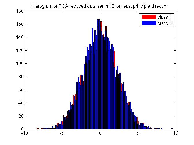
| − | + | <center>[[Image:Original data set in 2D.jpg|center]]<br> </center> <center>Figure 7. Original multivariate Gaussian distributed data set in 2D with equal probability. </center> <center>[[Image:Histogram of PCA-reduced data set in 1D on most principle direction.jpg|center]] </center> <center>Figure 8. Histogram of the PCA-reduced data after projection onto the most principle direction </center> <center>[[Image:Histogram of PCA-reduced data set in 1D on least principle direction.jpg|center]] </center> <center>Figure 9. Histogram of the PCA-reduced data after projection onto the least principle direction </center> | |
| − | <center>[[Image:Original data set in 2D.jpg|center]]<br> </center> | + | <br> |
| − | + | ||
| − | <center>Figure 7. Original data set in 2D | + | |
| − | + | ||
| − | <center>[[Image:Histogram of PCA-reduced data set in 1D on most principle direction.jpg|center]] </center> | + | |
| − | + | ||
| − | <center>Figure 8. Histogram of the PCA-reduced data onto the most principle direction </center> | + | |
| − | + | ||
| − | <center>[[Image:Histogram of PCA-reduced data set in 1D on least principle direction.jpg|center]] </center> | + | |
| − | + | ||
| − | <center>Figure 9. Histogram of the PCA-reduced data onto the least principle direction </center> | + | |
| − | <br> | + | |
<center> | <center> | ||
{| width="600" border="1" align="center" cellpadding="1" cellspacing="1" | {| width="600" border="1" align="center" cellpadding="1" cellspacing="1" | ||
| Line 165: | Line 135: | ||
| 49.45% | | 49.45% | ||
| 0.0062 | | 0.0062 | ||
| − | |}</center> | + | |} |
| − | + | </center> <center>Table 1. Performance of three methods. Look into tutorial for detail discussion. </center> | |
| − | <center>Table 1. Performance of three methods. Look into tutorial for detail discussion. </center> | + | <br> This approach is relatively straight forward, but it does not take into account how the distributions of each class are separated from each other after projecting onto the lower dimensional subspace. Therefore direct PCA may not be an optimal solution for the purpose of classification. Also, direct PCA is very sensitive to outlier data. Another approach is to define a measure of the spread of the distributions and find the transformation which maximizes this parameter. One such function is the ''Fisher linear discriminant''[4]. |
| − | + | ||
| − | <br> This approach is relatively straight forward, but it does not take into account how the distributions of each class are separated from each other after projecting onto the lower dimensional subspace. Therefore direct PCA may not be an optimal solution for the purpose of classification. Another approach is to define a measure of the spread of the distributions and find the transformation | + | |
== Discussion == | == Discussion == | ||
| − | PCA can throw out | + | PCA can throw out the less important information and can help reveal hidden, simplified dynamics in high dimensional data. It has broad application in signal processing, multivariate quality control, mechanical engineering, factor analysis, psychometrics, etc. |
| − | As we can see, PCA is a non-parametic analysis. There are no parameters or coefficients to adjust based on user experience. If one knows a-priori some features of the system, then it makes sense to incorporate those information into a parametric algorithm. But PCA can not provide us with such kind of | + | As we can see, PCA is a non-parametic analysis. There are no parameters or coefficients to adjust based on user experience. If one knows a-priori some features of the system, then it makes sense to incorporate those information into a parametric algorithm. But PCA can not provide us with such kind of flexibility. |
| − | Major extensions of PCA include: | + | '''Major extensions of PCA include:''' |
#Nonlinear generalizations: Kernal PCA uses techniques of kernel methods to perform the originally linear operations of PCA in a reproducing kernel Hilbert space with a non-linear mapping. | #Nonlinear generalizations: Kernal PCA uses techniques of kernel methods to perform the originally linear operations of PCA in a reproducing kernel Hilbert space with a non-linear mapping. | ||
#Multilinear generalizations: multilinear PCA (MPCA) extracts features directly from tensor representations. MPCA is solved by performing PCA in each mode of the tensor iteratively. MPCA is more efficient and better conditioned in practice and has been applied to face recognition, gait recognition, etc. | #Multilinear generalizations: multilinear PCA (MPCA) extracts features directly from tensor representations. MPCA is solved by performing PCA in each mode of the tensor iteratively. MPCA is more efficient and better conditioned in practice and has been applied to face recognition, gait recognition, etc. | ||
| − | #Robustness generalizations: weighted PCA increases robustness by assigning different weights to data objects based on their estimated relevancy to remove outlier, which is a sensitive resource to PCA performance | + | #Robustness generalizations: weighted PCA increases robustness by assigning different weights to data objects based on their estimated relevancy in order to remove outlier, which is a sensitive resource to direct PCA performance. |
#Non-Gaussian generalizations: Independent component analysis (ICA) is a computational method for separating a multivariate signal into additive subcomponents by assuming that the subcomponents are non-Gaussian signals and that they are all statistically independent from each other. | #Non-Gaussian generalizations: Independent component analysis (ICA) is a computational method for separating a multivariate signal into additive subcomponents by assuming that the subcomponents are non-Gaussian signals and that they are all statistically independent from each other. | ||
| − | #Probabilistic generalizations: | + | #Probabilistic generalizations: probabilistic PCA expresses PCA as the maximum likelihood solution of a probabilistic latent variable model. In this framework, Bayes and EM algorithm can be absorbed into PCA to solve more complex questions with higher efficiency. |
== References == | == References == | ||
| Line 193: | Line 161: | ||
---- | ---- | ||
| − | ==Questions and comments== | + | |
| − | If you have any questions, comments, etc. please post them on [[ | + | == Questions and comments == |
| + | |||
| + | If you have any questions, comments, etc. please post them on [[PCA comments|this page]]. | ||
| + | |||
---- | ---- | ||
| − | <br> | + | |
| + | <br> | ||
| + | |||
[[Category:ECE662]] [[Category:Bayes'_Theorem]] [[Category:Probability]] [[Category:Bayes'_Rule]] [[Category:Bayes'_Classifier]] [[Category:Slecture]] [[Category:ECE662Spring2014Boutin]] [[Category:ECE]] [[Category:Pattern_recognition]] | [[Category:ECE662]] [[Category:Bayes'_Theorem]] [[Category:Probability]] [[Category:Bayes'_Rule]] [[Category:Bayes'_Classifier]] [[Category:Slecture]] [[Category:ECE662Spring2014Boutin]] [[Category:ECE]] [[Category:Pattern_recognition]] | ||
Revision as of 17:41, 31 March 2014
Principle Component Analysis (PCA) tutorial
A slecture by Tian Zhou
(partially based on Prof. Mireille Boutin's ECE 662 lecture)
Contents
What will you learn from this slecture?
- A toy example to illustrate the idea of PCA
- The mathematical reasoning behind PCA
- A working example using PCA with Bayes rule in classification
- The strength and limitation of PCA and a brief introuction on various extensions of PCA
Prerequisite
This tutorial only requires a working knowledge of basic linear algebra. If you are familiar with standard deviation, covariance and eigen decompostion, then you are fine. Otherwise, Gilbert Strang's great book[1] is of great help.
Introduction
Principle Component Analysis (PCA) is a statistical method that uses orthonormal transformations to convert the observed correlated data into a set of linearly uncorrelated data, which are the so-called principle components. PCA has found numerous application fields like face recognition, dimension reduction, factor analysis and image compression, etc. Generally speaking, it's a common technique that can find certain patterns in high-dimension data, and by considering the most significant patterns only, it can reduce the computation efforts dramatically. When dealing with high-dimension data, it's always not easy for us to visualize the distribution of data, and thus it's very hard to find certain patterns from data which could potentially lead to a better design of classifier. PCA could help us in this case, to find the significant patterns.
This tutorial is divided into four sections
- A toy example of PCA
- Mathematical derivation of PCA
- Use PCA with Bayes rule in classification
- Discussion
A toy example
In this section, I will just use PCA on a simple data set to help you gain some intuition of PCA, the question of "why does it work" is not answered in this section, we just focus on "how to make it work". Then after you get hopefully some idea of PCA from this toy example, we will provide the mathematical derivation to explain why it works like this.
There are basically 6 steps in the procedure of using PCA, they are 1) Construct the data set, 2) Subtract the mean, 3) Calculate the covariance matrix, 4) Get eigenvalue decomposition of covariance matrix, 5) Choose the significant principle components, 6) Get the transformed data. Now we will go through all of them in detail.
Step 1: Construct the data set
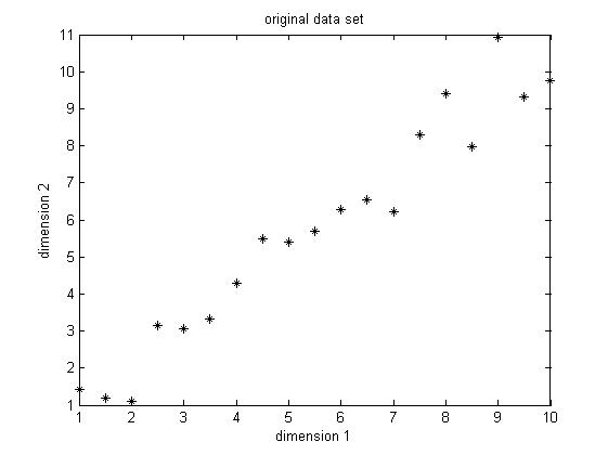
The data set I choose is only of two dimension, because it's easy for visualization. The original data set is shown below in Figure1. This is only a made-up data, there are 19 observations. As we can easily find, there is a positive correlation between data in the two dimensions.
Step 2: Subtract the mean
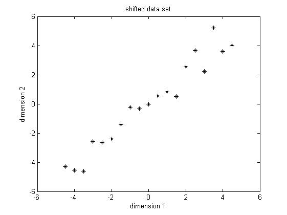
PCA requires the data set to have zero mean in each of the dimensions. Thus we have to subtract the mean, which is the sample average, in each dimension. The sample average for the data in dimension 1 is 5.5 and for data in dimension 2 is 5.7283. Then for the data in each dimension, we subtract the corresponding mean from the original data, the shifted data is shown in Figure 2. From now on, we will just refer the "shifted data" as "original data", unless stated explicitly.
Step 3: Calculate the covariance matrix
Since the data is two-dimensional, the covariance matrix should be a symmetric 2x2 matrix. The formula to calculate covariance is
,
N is the number of observations, notice that this is an unbiased estimate of the true covariance estimate, the derivation of this formula is beyond the scope of this tutorial. Using the above formula, we get the covariance
,
notice that the off-diagonal elements are positive, this implies a positive correlation between the data in the two dimensions, i.e., they will increase together.
Step 4: Get eigenvalue decomposition of the covariance matrix
Since the covariance matrix is symmetric and square, we can perform the eigenvalue decomposition and get a normalized eigenvector matrix and a diagonal eigenvalue matrix. They are
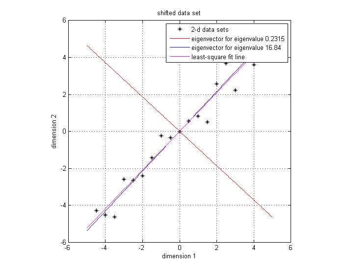
Notice that both eigen vectors are unitary vector, i.e. their length is 1. Now we plot the eigenvector together with data set in Figure 3. The red line indicates the direction of the eigenvector for the smaller eigenvalue, and the blue line indicates the direction of the eigenvector for the larger eigenvalue. First notice is that the two eigenvectors are perpendicular to each other , as expected. More importantly, the direction of the eignevector shows a significant pattern in the data set. It's easy to find out that the blue line goes through all the data points and it is a very good fit to the data. While the red line hardly reveals any trend of the distribution of data. To illustrate the phenomenon better, we also draw the line of best fit using least square regression in magenta. As we can see, the blue line and magenta line are very close to each other, both of them are a good fit for the data set.
Step 5: Choose the significant principle components
Now we come to the stage of choosing significant principle components. The originical data is in 2 dimension, and now we want to reduce it into 1 dimension. Notice that a 1 dimensional data will form a line in 2D space. So reduce the data from 2D to 1D could also be interpreted as projecting the original data sets onto a line, and this line could preserve the most amount of information of the original 2D data set. Notice that we can't preserve all the information after projection, we can only compress the original information and represent it in a lower dimension, which could be still useful in some sense. Here we define the sum of square distances between the original data set and the projected data set as the error of the projection, or as a measure of loss of information. Since now from the eigen decomposition of the covariance matrix, we get two vectors which represent two lines, we will just blindly follow these lines and project our original data set onto them, then compare the loss of information after the projection. Here we will define the direction which is decided by the eigenvector as "principle direction".
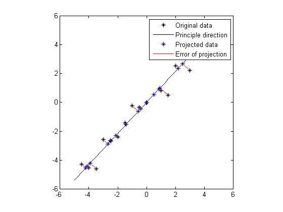
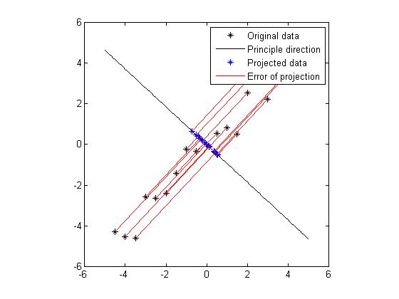
Figure 4 and Figure 5 show the projection for these two principle directions, respectively. In each figure, the black dots are the original data set, the black line shows the direction of the eigenvector, the blue dots are the points which are projections from the original data onto the principle direction. And the red line indicates the distance between the original data and the projected data, hence the error of the projection. We would like to find a way of projection which could minimize the total error. Obviously, from the figure we know that the projection onto the direction which is specified by the eigenvector of the larger eigenvalue is favored. In fact, the sum of errors of projection in Figure 4 is 7.17 and the sum of errors of projection in Figure 5 is 64.6. Without doubt, if we want to project the original data from 2D to 1D, we will choose the eigenvector or the larger eigenvalue as projection axis. Now we get an intuition that the eigenvectors which correspond to larger eigenvalues could provide more significant patterns of the data, thus could be chosen to generate significant principle components.
In general, the procedure to choose the significant principle components contain the following steps: 1) get the eigendecomposition of the covariance matrix, 2) sort the eigenvalues in decreasing order, and swap the eigenvectors correspondly, 3) choose the largest p eigenvalues and the corresponding eigenvectors to serve as a basis for the new space which the reduced or compressed data lie in. The value of p is chosen based on a user-definied criterion, like the sum of energy should be at least 90% of the original energy, or the sum or error could not exceed a threshold, 4) stack these eigenvectors to form a feature vector, which serves as the basis for the reduced space.
Step 6: Get the transformed data
Notice that after the projection, the projected data are still in 2D. And we have not really compressed the data yet. To accomplish that, we need to rotate the line and put the line in 1D, so that the reduced data is represented by only one variable. Actually the projection and rotation could be combined into one step only, that is to multiply the original data by the feature vector. The formula is
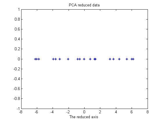
Based on the organization of the original data, we might need to transpose the OriginalData matrix, just to make sure that the matrix multiplication could enjoy the right size of each matrix. In Figure 6, the reduced data is shown. It's only a line (1D data) shown in 2D. As we can see, this is the rotation of the projection in Figure 4. To get the original data back, we notice that the featurevector matrix is orthonorma, thus we have the formula,
Throughout this section, I illustrated a toy example of PCA to give you a general idea and hopefully some intuition of how PCA works. After we use PCA to reduce the data from original dimension to a lower dimension, we could use this compressed data set as an efficient representation of the original data, and further could make some decision making processing based on this reduced data set to save computational resources. In the next section we will focus more on the mathematical theories behind PCA, trying to explain why it works.
Mathematical derivation
In this chapter we will explore the mathematical theories behind PCA to understand why it works. PCA can be defined as the orthogonal projection of the data onto a lower dimensional linear space, known as the principle subspace, such that the variance of the projected data is maximized[3] (other definition and derivation of PCA could be found in [4]). Following this idea of maximizing variance, let's derive the formula for PCA.
The dataset contains observations xn, where n = 1,...,N, and xn is a variable with dimension M. Our goal is to project the data onto a subspace which has dimension P < M while maximizing the variance of the projected data. For now we will assume that P is given, i.e. we are already given the dimension of the subspace.
First, let's consider the projection onto a one-dimensional space (P = 1). To define the direction of this subspace, we use a M-dimensional unit vector u1 so that $ u_1^Tu_1 = 1 $ , this is for convenience and without loss of generality. Notice that here only the direction defined by u1 is of interest to us, the magnitude of u1 is not critical. After we define the direction of the subspace, each data point xn is projected onto this subspace, and we get a scalar $ u_1^Tx_n $ as the result of each projection. The mean of the projected data is $ u_1^T\bar{x} $ , where $ \bar{x} $ is the sample mean of the original data set given by
and the variance of the projected data which lies in the subspace is given by
where S is the data covariance matrix defined by
Again, notice that this is an unbiased covariance matrix. We now need to maximize the variance $ u_1^TSu_1 $ of the projected data with respect to u1. The constraint comes from the normalization condition $ u_1^Tu_1=1 $. Recall that only the direction matters, the magnitude is not critical. To enforce this constraint, we bring a Lagrange multiplier that we can denote as λ1, and then make an unconstrained maximization of
we get the derivative of L with respect to u1 and set it to zero
we get
from the above equation we got the conclusion that 1) u1 must be an eigenvector of S; 2) the variance will be a maximum when we set u1 equal to the eigenvector of the largest eigenvalue λ1. This eigenvector is know as the first principal component. We can define additional principle components in an induction fashion. Choose each new direction to be that which maximizes the projected covariance among all possible directions orthogonal to those already considered. If we consider the general case of an P-dimensional projection space, the optimal linear projection for which the variance of the projected data is maximized is defined by the P eigenvectors u1,...,uP of the data covariance matrix S, corresponding to the P largest eigenvalues λ1,...,λP.
Use PCA with Bayes rule in classification
In this section, we will use PCA with Bayes rule to classify synthesized 2D data. We will compare the performance of classification between two methods: 1) directly use Bayes rule to classify 2D data; 2) first use PCA to reduce the dimension of data to 1D, then apply Bayes rule to classify the projected data.
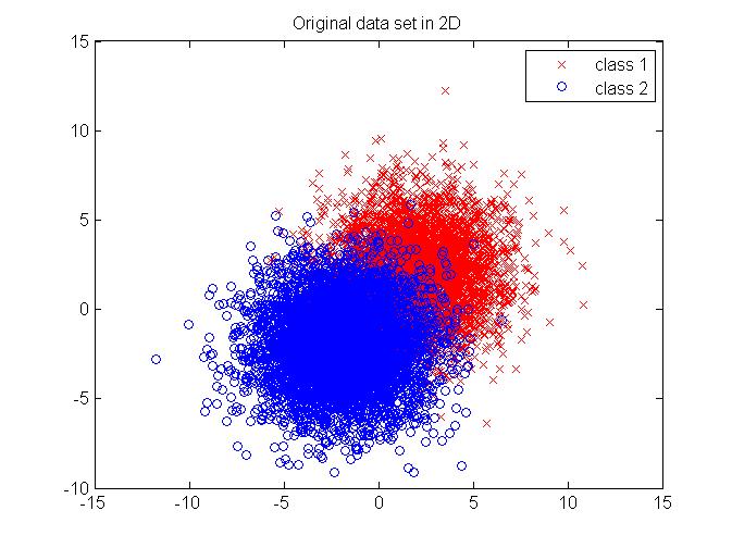
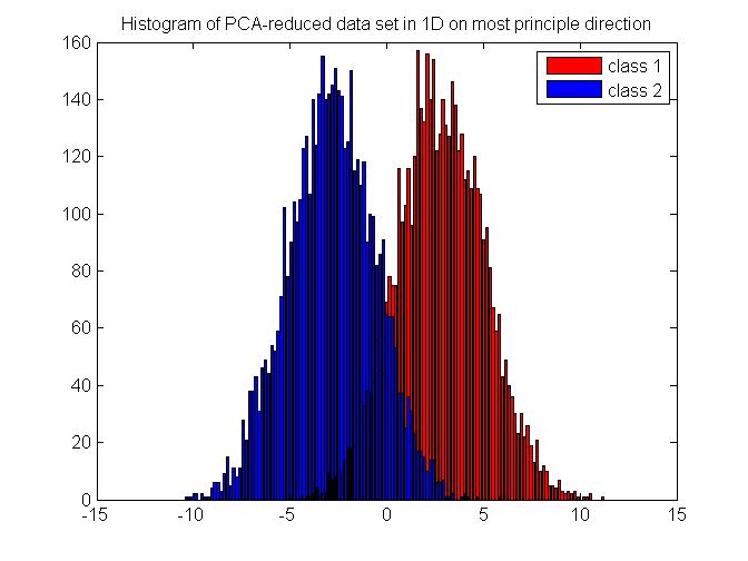
We will generate synthesized data which follows a multivariate Gaussian distribution in 2D. The data comes from two random seed which are of equal probability and are well separated for better illustration. The original data set in 2D is shown in Figure 7. First, we apply Bayes rule on the 2D data directly and get a classification result. Then, we use PCA to reduce the data into 1D, and then perform Bayes rule on the projected data set. The histogram of the projected data is shown in Figure 8. For the purpose of comparison, we also show the histogram of the data which are projected onto the least principle direction in Figure 9 and perform Bayes rule for classification, too. The results are shown in Table 1. As we can see, performing Bayes rule on the PCA-reduced data on the most principle direction generates a same-level error rate, with only about 2% of calculation time, compared with the original method using Bayes rule on 2D data directly. Performing Bayes rule on the PCA-reduced data on the least principle direction generates an error rate of 50%, which is no different from just using priors, thus proving the lack of discrimination nature on this projection axis.
| Methods | Error Rate | Time/s |
| Bayes rule in 2D | 9.87% | 0.292 |
| Bayes rule in 1D (projected onto most principle direction) | 9.84% | 0.0071 |
| Bayes rule in 1D (projected onto least principle direction) | 49.45% | 0.0062 |
This approach is relatively straight forward, but it does not take into account how the distributions of each class are separated from each other after projecting onto the lower dimensional subspace. Therefore direct PCA may not be an optimal solution for the purpose of classification. Also, direct PCA is very sensitive to outlier data. Another approach is to define a measure of the spread of the distributions and find the transformation which maximizes this parameter. One such function is the Fisher linear discriminant[4].
Discussion
PCA can throw out the less important information and can help reveal hidden, simplified dynamics in high dimensional data. It has broad application in signal processing, multivariate quality control, mechanical engineering, factor analysis, psychometrics, etc.
As we can see, PCA is a non-parametic analysis. There are no parameters or coefficients to adjust based on user experience. If one knows a-priori some features of the system, then it makes sense to incorporate those information into a parametric algorithm. But PCA can not provide us with such kind of flexibility.
Major extensions of PCA include:
- Nonlinear generalizations: Kernal PCA uses techniques of kernel methods to perform the originally linear operations of PCA in a reproducing kernel Hilbert space with a non-linear mapping.
- Multilinear generalizations: multilinear PCA (MPCA) extracts features directly from tensor representations. MPCA is solved by performing PCA in each mode of the tensor iteratively. MPCA is more efficient and better conditioned in practice and has been applied to face recognition, gait recognition, etc.
- Robustness generalizations: weighted PCA increases robustness by assigning different weights to data objects based on their estimated relevancy in order to remove outlier, which is a sensitive resource to direct PCA performance.
- Non-Gaussian generalizations: Independent component analysis (ICA) is a computational method for separating a multivariate signal into additive subcomponents by assuming that the subcomponents are non-Gaussian signals and that they are all statistically independent from each other.
- Probabilistic generalizations: probabilistic PCA expresses PCA as the maximum likelihood solution of a probabilistic latent variable model. In this framework, Bayes and EM algorithm can be absorbed into PCA to solve more complex questions with higher efficiency.
References
- Gilbert Strang, "Introduction to Linear Algebra", Wellesley-Cambridge Press, February 2009. ISBN: 9780980232714
- Mireille Boutin, "ECE662: Statistical Pattern Recognition and Decision Making Processes," Purdue University, Spring 2014.
- Hotelling, H. (1933). Analysis of a complex of statistical variables into principal components. Journal of educational psychology, 24(6), 417.
- Bishop, C. M. (2006). Pattern recognition and machine learning (Vol. 1, p. 740). New York: springer.
Questions and comments
If you have any questions, comments, etc. please post them on this page.

