| Line 19: | Line 19: | ||
== Prerequisite == | == Prerequisite == | ||
| − | This tutorial only requires a working knowledge of baisc linear algebra. If you are familar with standard deviation, covariance and eigen decompostion, then you are fine. If not, Gilbert Strang wrote a great book<sup>[1]</sup>, which is of great help.<br> | + | This tutorial only requires a working knowledge of baisc linear algebra. If you are familar with standard deviation, covariance and eigen decompostion, then you are fine. If not, Gilbert Strang wrote a great book<sup>[1]</sup>, which is of great help.<br> |
---- | ---- | ||
| Line 25: | Line 25: | ||
== Introduction == | == Introduction == | ||
| − | Principle Component Analysis (PCA) is a statistical method that uses orthonormal transformations to convert the observed correlated data into a set of linearly uncorrelated data, which are the so-called principle components. PCA has found numerous application fields like face recognition, dimension reduction, factor analysis and image compression, etc. Generally speaking, it's a common technique that can find certain patterns in high-dimension data, and thus can reduce the computation efforts by only considering a certain set of significant patterns. When dealing with high-dimension data, it's always not easy for us to visualize the distribution of data, and thus it's very hard to find certain patterns from data which could lead to a better desigh of classifier. PCA could help us in this case, to find the significant patterns. | + | Principle Component Analysis (PCA) is a statistical method that uses orthonormal transformations to convert the observed correlated data into a set of linearly uncorrelated data, which are the so-called principle components. PCA has found numerous application fields like face recognition, dimension reduction, factor analysis and image compression, etc. Generally speaking, it's a common technique that can find certain patterns in high-dimension data, and thus can reduce the computation efforts by only considering a certain set of significant patterns. When dealing with high-dimension data, it's always not easy for us to visualize the distribution of data, and thus it's very hard to find certain patterns from data which could lead to a better desigh of classifier. PCA could help us in this case, to find the significant patterns. |
This tutoril is divided into three sections | This tutoril is divided into three sections | ||
| Line 35: | Line 35: | ||
== A toy example == | == A toy example == | ||
| − | In this section, I will just use PCA on a simple data set to helo you gain some intuition of PCA, the question of "why does it work" is not answered in this section, we just focus on "how to make it work". Then after you get enough intuition from this toy example, you can decide whether PCA will work fine in your application scenario. The mathematical derivation will come later. | + | In this section, I will just use PCA on a simple data set to helo you gain some intuition of PCA, the question of "why does it work" is not answered in this section, we just focus on "how to make it work". Then after you get enough intuition from this toy example, you can decide whether PCA will work fine in your application scenario. The mathematical derivation will come later. |
| − | There are basically 6 steps in the procedure of using PCA, they are 1) Construct the data set, 2) Subtract the mean, 3) Calculate the covariance matrix, 4) Get eigenvalue decomposition of covariance matrix, 5) Choose the significant principle components, 6) Get the transformed data. Now we will go through all of them in detail. | + | There are basically 6 steps in the procedure of using PCA, they are 1) Construct the data set, 2) Subtract the mean, 3) Calculate the covariance matrix, 4) Get eigenvalue decomposition of covariance matrix, 5) Choose the significant principle components, 6) Get the transformed data. Now we will go through all of them in detail. |
| − | <font size="2">''' | + | === <font size="2">'''Step 1: Construct the data set'''</font> === |
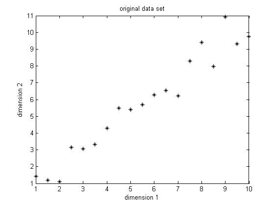
| − | The data set I choose is only two dimension, because it's easier for visualization. The original data set is shown below in Figure1. This is only a made-up data, there are 19 observations. As we can easily find, there is a positive correlation between the two dimensions. | + | The data set I choose is only two dimension, because it's easier for visualization. The original data set is shown below in Figure1. This is only a made-up data, there are 19 observations. As we can easily find, there is a positive correlation between the two dimensions. |
[[Image:New Original data.jpg|center]]<br> | [[Image:New Original data.jpg|center]]<br> | ||
| − | Figure 1. Original data set, data dimension is 2, 19 observations | + | Figure 1. Original data set, data dimension is 2, 19 observations |
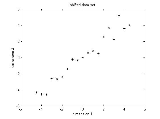
| − | <font size="2">''' | + | <font size="2">'''Step 2: Subtract the mean'''</font><br> PCA requires the data set to have zero mean in each of the dimensions so that it can work properly. Thus we have to subtract the mean, which is the sample average, in each dimension. It's not hard to find out that the sample average for the data in dimension 1 is 5.5 and for data in dimension 2 is 5.7283. Then for data in each dimension, we subtract the correponding mean, the result shifted data is shown in Figure 2. |
[[Image:New Shifted data.jpg|center]]<br> | [[Image:New Shifted data.jpg|center]]<br> | ||
| − | Figure 2. Shifted data set, subtract the sample average for each dimension | + | Figure 2. Shifted data set, subtract the sample average for each dimension |
| − | ''' | + | '''Step 3: Calculate the covariance matrix''' |
| − | Since the data is two-dimensional, the covariance matrix should be a symmetric 2x2 matrix. The formula to calculate covariance is <math> \sigma_(x,y) = \frac{1}{N-1}\textbf{x}^T \textbf{y} </math>, N is the number of observations, notice that this is an unbiased estimate of the true covariance estimate, the derivation of this formula is beyond the scope of this tutorial. After the easy calculation, we get <math> Cov = \begin{bmatrix} 7.9167 & 8.2813 \\[0.3em] 8.2813 & 9.1552 \end{bmatrix}</math>, notice that the off-diagonal elements are positive, this implies a positive correlation between the data in the two dimensions. They will increase together. | + | Since the data is two-dimensional, the covariance matrix should be a symmetric 2x2 matrix. The formula to calculate covariance is <math> \sigma_(x,y) = \frac{1}{N-1}\textbf{x}^T \textbf{y} </math>, N is the number of observations, notice that this is an unbiased estimate of the true covariance estimate, the derivation of this formula is beyond the scope of this tutorial. After the easy calculation, we get <math> Cov = \begin{bmatrix} 7.9167 & 8.2813 \\[0.3em] 8.2813 & 9.1552 \end{bmatrix}</math>, notice that the off-diagonal elements are positive, this implies a positive correlation between the data in the two dimensions. They will increase together. |
| − | ''' | + | '''Step 4: Get eigenvalue decomposition of the covariance matrix''' |
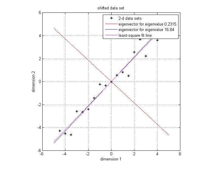
| − | Since the covariance matrix is symmetric and square, we can perform the eigenvalue decomposition and get a normalized eigenvector matrix and a diagonal eigenvalue matrix. They are <math> Eigenvector = \begin{bmatrix} -0.7330 & 0.6802 \\[0.3em] 0.6802 & 0.7330 \end{bmatrix} Eigenvalue = \begin{bmatrix} 0.2315 \\[0.3em] 16.8404 \end{bmatrix}</math> Notice that both eigen vectors are unitary vector, i.e. their length is 1. Now we plot the eigenvector together with data set in Figure 3. The red line | + | Since the covariance matrix is symmetric and square, we can perform the eigenvalue decomposition and get a normalized eigenvector matrix and a diagonal eigenvalue matrix. They are <math> Eigenvector = \begin{bmatrix} -0.7330 & 0.6802 \\[0.3em] 0.6802 & 0.7330 \end{bmatrix} Eigenvalue = \begin{bmatrix} 0.2315 \\[0.3em] 16.8404 \end{bmatrix}</math> Notice that both eigen vectors are unitary vector, i.e. their length is 1. Now we plot the eigenvector together with data set in Figure 3. The red line indicates the direction for the eigenvector for the smaller eigenvalue, and the blue line ind the direction for the eigenvector for the larger eigenvalue. First notice is that the two eigenvectors are perpendicular to each other, as expected. Then, more importantly, the direction of the eignevector shows a siginicant pattern in the data set. It's easy to find out that the blue line goes through all the data points and it is a very good fit to the data. To illustrate the phenomenon better, I also drew the line in magenta of best fit using least square regression. As we can see, the blue line and magenta line are very close to each other.<br> |
| − | + | [[Image:Eigenvector.jpg|center]] | |
| − | Figure 3. Data set, eigen vector and the best-fit line using least square | + | Figure 3. Data set, eigen vector and the best-fit line using least square |
| + | '''Step 5: Choose the significant principle components''' | ||
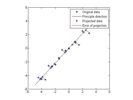
| + | Now we come to the stage of choosing significant principle components. The originical data is in 2 dimension, and now we want to reduce it into 1 dimension. Notice that a 1 dimensional data will form a line in 2D space. So reduce the data from 2D to 1D could also be interpreted as projectiong all the original data sets onto a line, and this line could preserve the most amount of information of the original 2D dataset. Notice that we can't preserve all the information after projection, we can only compress the originical information and represent it in a lower dimension, which could be still useful in some sense. Here we define sum of square distances between the original dataset and the projected dataset as the error of the projection, or as a measure of loss of information. Since now from the eigen decomposition of the covariance matrix, we get two vectors whichrepresent two lines, we will just blindly follow this idea and project our original dataset onto these two lines and compare the loss of information after the projection. Here we will define the direction which is decided by the eigenvector as "principle direction". Figure 4 and Figure 5 show the projection for these two principle directions, respectively. In each figure, the black dots are the original data set, the black line indicates the line which is decided by the eigenvector, the blue dots are the points which are projections onto the principle direction. And the red line indicates the distance between the original data and the projected data, hence the error of the projection. We would like to find a way of projection which could minimize the total error. Obviously, from the figure we know that the projection along the direction which is speficied by the eigenvector of the larger eigenvalue is favored. In fact, the sum of errors in Figure 4 is 7.17 is and the sum of errors in Figure 5 is 64.6. Without doubt, if we want to project the original data from 2D to 1D, we will choose the direction in Figure 4 as projection axis. Now we get a intuition that the eigenvectors which correspond to larger eigenvalues could provide more significant patterns of the data, thus could be chosen as significant principle components. | ||
| + | |||
| + | In general, the procedures to choose the significant principle components are like these: 1) get the eigendecomposition of the covariance matrix, 2) sort the eigenvalues from large to small, and swap the eigenvectors correspondly, 3) choose the largest p eigenvalues and the corresponding eigenvectors to serve as a basis for the new space which the reduced or compressed data would lie in, the principle of choosing p is based on a user-definied criterion, like the sum of energy should be at least 90% of the original energy, or the sum or error could not exceed a threshold, 4) stack these eigenvectors to form a feature vector, which serves as the basis for the reduced space. <math> FeatureVector = \begin{bmatrix} EigenVec 1 & EigenVec 2 & ... & EigenVec P\end{bmatrix} </math> | ||
| + | |||
| + | [[Image:Projection large evalue.jpg|center]] | ||
| + | |||
| + | Figure 4: Projection onto the eigenvector which corresponds to the '''large '''eigenvalue. | ||
| + | |||
| + | [[Image:Projection small evalue.jpg|center]] | ||
| + | |||
| + | Figure 5: Projection onto the eigenvector which corresponds to the '''small '''eigenvalue | ||
| + | |||
| + | <br> | ||
| + | |||
| + | '''Step 6: Get the transformed data''' | ||
| + | |||
| + | Notice that after the projection, the projected data are still in 2D. And we have not really compressed the data yet. To accomplish that, we need to rotate the line and put the line in 1D. Actually the projection and rotation could be combined into one step only, that is to multiply the original data by the feature vector. The formula is '''''ReducedData = OriginalData*FeatureVecotor'''''. Based on the organization of the original data, we might need to transpose the OriginalData matrix, just to make sure that the matrix multiplication could enjoy the right size of each matrix. In Figure 6, the reduced data is shown. It's only a line (1D data) shown in 2D. As we can see, this is the rotation of the projection in Figure 4. To get the original data back, it's very easy. Follow the formula above, '''''OriginalData = ReducedData*FeatureVector<sup>T</sup>''''', since the featurevector is an orthonormal matrix. <sup></sup><br> | ||
| + | |||
| + | [[Image:PCA reduced data.jpg|center]] | ||
| + | |||
| + | Figure 6: The PCA reduced data, it's only 1D data but shown in 2D. | ||
| + | |||
| + | <br> | ||
| + | |||
| + | Throughout this section, I illustrated a toy example of PCA to give you a general idea and hopefully some intuition of how PCA works. After we use PCA to reduce the data from original dimension to a lower dimension, we could use this compressed dataset as an efficient representation of the original data, or could make some decision making processing based on this reduced dataset to save computational resources. In the next section we will focus more on the mathematic theories behind PCA, trying to explain why it works. | ||
| + | |||
| + | == <br>Mathematical derivation == | ||
| + | |||
| + | In this chapter we will explore the mathematical theories behind PCA to understand why it works. The data set is <span class="texhtml">''X''</span>, an <math> m \times n </math> matrix, where <span class="texhtml">''m''</span> is the number of observations and <span class="texhtml">''n''</span> is the dimension of original data. PCA can be defined as the orthogonal projection of the data onto a lower dimensional linear space, known as the ''principle subspace'', such that the variance of the projected data is maximized<sup>[3]</sup> | ||
| + | |||
| + | <br> | ||
| + | |||
| + | <br> | ||
---- | ---- | ||
| Line 72: | Line 106: | ||
#Gilbert Strang, "Introduction to Linear Algebra", Wellesley-Cambridge Press, February 2009. ISBN: 9780980232714 | #Gilbert Strang, "Introduction to Linear Algebra", Wellesley-Cambridge Press, February 2009. ISBN: 9780980232714 | ||
| − | #[https://engineering.purdue.edu/~mboutin/ Mireille Boutin], "ECE662: Statistical Pattern Recognition and Decision Making Processes," Purdue University, Spring 2014. | + | #[https://engineering.purdue.edu/~mboutin/ Mireille Boutin], "ECE662: Statistical Pattern Recognition and Decision Making Processes," Purdue University, Spring 2014. |
| + | #Hotelling, H. (1933). Analysis of a complex of statistical variables into principal components. Journal of educational psychology, 24(6), 417. | ||
---- | ---- | ||
Revision as of 08:03, 25 March 2014
Principle Component Analysis (PCA) tutorial
A slecture by Tian Zhou
(partially based on Prof. Mireille Boutin's ECE 662 lecture)
Contents
What will you learn from this slecture?
- A toy example of using PCA to gain some intuition behind the method
- The mathematical reasoning behind this approach
- The strength and limitation of PCA and potential working field
Prerequisite
This tutorial only requires a working knowledge of baisc linear algebra. If you are familar with standard deviation, covariance and eigen decompostion, then you are fine. If not, Gilbert Strang wrote a great book[1], which is of great help.
Introduction
Principle Component Analysis (PCA) is a statistical method that uses orthonormal transformations to convert the observed correlated data into a set of linearly uncorrelated data, which are the so-called principle components. PCA has found numerous application fields like face recognition, dimension reduction, factor analysis and image compression, etc. Generally speaking, it's a common technique that can find certain patterns in high-dimension data, and thus can reduce the computation efforts by only considering a certain set of significant patterns. When dealing with high-dimension data, it's always not easy for us to visualize the distribution of data, and thus it's very hard to find certain patterns from data which could lead to a better desigh of classifier. PCA could help us in this case, to find the significant patterns.
This tutoril is divided into three sections
- A toy example
- Mathematical derivation
- Discusssion
A toy example
In this section, I will just use PCA on a simple data set to helo you gain some intuition of PCA, the question of "why does it work" is not answered in this section, we just focus on "how to make it work". Then after you get enough intuition from this toy example, you can decide whether PCA will work fine in your application scenario. The mathematical derivation will come later.
There are basically 6 steps in the procedure of using PCA, they are 1) Construct the data set, 2) Subtract the mean, 3) Calculate the covariance matrix, 4) Get eigenvalue decomposition of covariance matrix, 5) Choose the significant principle components, 6) Get the transformed data. Now we will go through all of them in detail.
Step 1: Construct the data set
The data set I choose is only two dimension, because it's easier for visualization. The original data set is shown below in Figure1. This is only a made-up data, there are 19 observations. As we can easily find, there is a positive correlation between the two dimensions.
Figure 1. Original data set, data dimension is 2, 19 observations
Step 2: Subtract the mean
PCA requires the data set to have zero mean in each of the dimensions so that it can work properly. Thus we have to subtract the mean, which is the sample average, in each dimension. It's not hard to find out that the sample average for the data in dimension 1 is 5.5 and for data in dimension 2 is 5.7283. Then for data in each dimension, we subtract the correponding mean, the result shifted data is shown in Figure 2.
Figure 2. Shifted data set, subtract the sample average for each dimension
Step 3: Calculate the covariance matrix
Since the data is two-dimensional, the covariance matrix should be a symmetric 2x2 matrix. The formula to calculate covariance is $ \sigma_(x,y) = \frac{1}{N-1}\textbf{x}^T \textbf{y} $, N is the number of observations, notice that this is an unbiased estimate of the true covariance estimate, the derivation of this formula is beyond the scope of this tutorial. After the easy calculation, we get $ Cov = \begin{bmatrix} 7.9167 & 8.2813 \\[0.3em] 8.2813 & 9.1552 \end{bmatrix} $, notice that the off-diagonal elements are positive, this implies a positive correlation between the data in the two dimensions. They will increase together.
Step 4: Get eigenvalue decomposition of the covariance matrix
Since the covariance matrix is symmetric and square, we can perform the eigenvalue decomposition and get a normalized eigenvector matrix and a diagonal eigenvalue matrix. They are $ Eigenvector = \begin{bmatrix} -0.7330 & 0.6802 \\[0.3em] 0.6802 & 0.7330 \end{bmatrix} Eigenvalue = \begin{bmatrix} 0.2315 \\[0.3em] 16.8404 \end{bmatrix} $ Notice that both eigen vectors are unitary vector, i.e. their length is 1. Now we plot the eigenvector together with data set in Figure 3. The red line indicates the direction for the eigenvector for the smaller eigenvalue, and the blue line ind the direction for the eigenvector for the larger eigenvalue. First notice is that the two eigenvectors are perpendicular to each other, as expected. Then, more importantly, the direction of the eignevector shows a siginicant pattern in the data set. It's easy to find out that the blue line goes through all the data points and it is a very good fit to the data. To illustrate the phenomenon better, I also drew the line in magenta of best fit using least square regression. As we can see, the blue line and magenta line are very close to each other.
Figure 3. Data set, eigen vector and the best-fit line using least square
Step 5: Choose the significant principle components
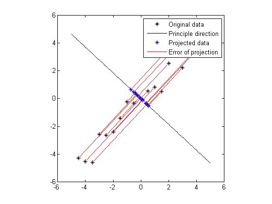
Now we come to the stage of choosing significant principle components. The originical data is in 2 dimension, and now we want to reduce it into 1 dimension. Notice that a 1 dimensional data will form a line in 2D space. So reduce the data from 2D to 1D could also be interpreted as projectiong all the original data sets onto a line, and this line could preserve the most amount of information of the original 2D dataset. Notice that we can't preserve all the information after projection, we can only compress the originical information and represent it in a lower dimension, which could be still useful in some sense. Here we define sum of square distances between the original dataset and the projected dataset as the error of the projection, or as a measure of loss of information. Since now from the eigen decomposition of the covariance matrix, we get two vectors whichrepresent two lines, we will just blindly follow this idea and project our original dataset onto these two lines and compare the loss of information after the projection. Here we will define the direction which is decided by the eigenvector as "principle direction". Figure 4 and Figure 5 show the projection for these two principle directions, respectively. In each figure, the black dots are the original data set, the black line indicates the line which is decided by the eigenvector, the blue dots are the points which are projections onto the principle direction. And the red line indicates the distance between the original data and the projected data, hence the error of the projection. We would like to find a way of projection which could minimize the total error. Obviously, from the figure we know that the projection along the direction which is speficied by the eigenvector of the larger eigenvalue is favored. In fact, the sum of errors in Figure 4 is 7.17 is and the sum of errors in Figure 5 is 64.6. Without doubt, if we want to project the original data from 2D to 1D, we will choose the direction in Figure 4 as projection axis. Now we get a intuition that the eigenvectors which correspond to larger eigenvalues could provide more significant patterns of the data, thus could be chosen as significant principle components.
In general, the procedures to choose the significant principle components are like these: 1) get the eigendecomposition of the covariance matrix, 2) sort the eigenvalues from large to small, and swap the eigenvectors correspondly, 3) choose the largest p eigenvalues and the corresponding eigenvectors to serve as a basis for the new space which the reduced or compressed data would lie in, the principle of choosing p is based on a user-definied criterion, like the sum of energy should be at least 90% of the original energy, or the sum or error could not exceed a threshold, 4) stack these eigenvectors to form a feature vector, which serves as the basis for the reduced space. $ FeatureVector = \begin{bmatrix} EigenVec 1 & EigenVec 2 & ... & EigenVec P\end{bmatrix} $
Figure 4: Projection onto the eigenvector which corresponds to the large eigenvalue.
Figure 5: Projection onto the eigenvector which corresponds to the small eigenvalue
Step 6: Get the transformed data
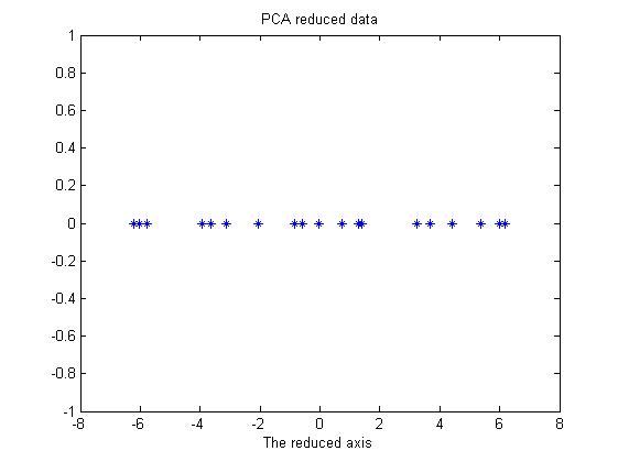
Notice that after the projection, the projected data are still in 2D. And we have not really compressed the data yet. To accomplish that, we need to rotate the line and put the line in 1D. Actually the projection and rotation could be combined into one step only, that is to multiply the original data by the feature vector. The formula is ReducedData = OriginalData*FeatureVecotor. Based on the organization of the original data, we might need to transpose the OriginalData matrix, just to make sure that the matrix multiplication could enjoy the right size of each matrix. In Figure 6, the reduced data is shown. It's only a line (1D data) shown in 2D. As we can see, this is the rotation of the projection in Figure 4. To get the original data back, it's very easy. Follow the formula above, OriginalData = ReducedData*FeatureVectorT, since the featurevector is an orthonormal matrix.
Figure 6: The PCA reduced data, it's only 1D data but shown in 2D.
Throughout this section, I illustrated a toy example of PCA to give you a general idea and hopefully some intuition of how PCA works. After we use PCA to reduce the data from original dimension to a lower dimension, we could use this compressed dataset as an efficient representation of the original data, or could make some decision making processing based on this reduced dataset to save computational resources. In the next section we will focus more on the mathematic theories behind PCA, trying to explain why it works.
Mathematical derivation
In this chapter we will explore the mathematical theories behind PCA to understand why it works. The data set is X, an $ m \times n $ matrix, where m is the number of observations and n is the dimension of original data. PCA can be defined as the orthogonal projection of the data onto a lower dimensional linear space, known as the principle subspace, such that the variance of the projected data is maximized[3]
References
- Gilbert Strang, "Introduction to Linear Algebra", Wellesley-Cambridge Press, February 2009. ISBN: 9780980232714
- Mireille Boutin, "ECE662: Statistical Pattern Recognition and Decision Making Processes," Purdue University, Spring 2014.
- Hotelling, H. (1933). Analysis of a complex of statistical variables into principal components. Journal of educational psychology, 24(6), 417.
Questions and comments
If you have any questions, comments, etc. please post them on this page.

