(Updated Conditional Probability statement as per Professor's Email) |
|||
| (75 intermediate revisions by 4 users not shown) | |||
| Line 1: | Line 1: | ||
Probability : Group 4 | Probability : Group 4 | ||
| − | Kalpit Patel | + | Kalpit Patel, |
| − | Rick Jiang | + | Rick Jiang, |
| − | Bowen Wang | + | Bowen Wang, |
Kyle Arrowood | Kyle Arrowood | ||
| − | + | Probability | |
| − | + | Definition: Probability is a measure of the likelihood of an event to occur. Many events cannot be predicted with total certainty. We can predict only the chance of an event to occur i.e., how likely they are going to happen, using it. | |
| − | + | ||
| − | + | ||
| − | Definition: Probability is a measure of the likelihood of an event to occur. Many events cannot be predicted with total certainty. We can predict only the chance of an event to occur i.e., how likely they are going to happen, using it | + | |
Notation: | Notation: | ||
| − | 1) Sample space (S): Set of all possible outcomes of | + | 1) Sample space (S): Set of all possible outcomes of any random experiment. |
| − | 2) Event: Any subsets of outcomes | + | 2) Event: Any subsets of outcomes contained in the sample space S. |
| − | + | Mutually exclusivity: | |
| − | + | When events A and B have no outcomes in common [[File:Screen_Shot_2022-11-15_at_10.56.42.png|130px|]] | |
| − | |||
| − | + | Axioms of probability: | |
| + | 1. Probability can range from 0 to 1, where 0 means the event to be an impossible one and 1 indicates a certain event. -> [[File:Screen_Shot_2022-11-22_at_11.20.02.png|200px|]] | ||
| − | + | 2. The probability of all the events in a sample space adds up to 1. -> P(S) = 1 | |
| − | [[File: | + | 3. When all events have no outcomes in common. |
| + | -> [[File:Probility.png|400px|]] | ||
| + | Properties of probability function: | ||
| + | 1. P(A^c) = 1 - P(A). The subset of outcomes in the sample space and are not in the event. Either event or its complement will happen, but not both. | ||
| − | + | 2. If A and B are mutually exclusive then P(A∧B) = 0. No common outcome. | |
| + | |||
| + | 3. P(A∨B) = P(A) + P(B) - P(A∧B). When A and B are not mutually exclusive, it needs to subtract the probability of common event because the occasions on which A and B both occur are counted twice. | ||
| + | |||
| + | |||
| + | Conditional Probability: | ||
| + | |||
| + | Conditional probability is defined as the likelihood of an event or outcome occurring, based on the occurrence of a previous event or outcome. It is the measure of the probability of an event A, given that another event B has already occurred. | ||
| + | |||
| + | [[File:cond4.png|300x300px|center]] | ||
| + | |||
| + | [[File:gfg2.png|300x300px|center]] | ||
| + | |||
| + | When P(B) is '''not''' zero, then we can write the formula in the quotient form and visualize the conditional probability as a ratio. | ||
| + | |||
| + | |||
| + | |||
| + | Independent Events: | ||
| + | |||
| + | This is a special case of Conditional Probability, where the occurrence of one event does not affect the probability of another event. In other words, for two events A and B: | ||
| + | [[File:inde3.png|300x300px|center]] | ||
| + | |||
| + | Bayes' Theorem Definition: | ||
| + | |||
| + | [[File:Bayes-def.png|400px|]] | ||
| + | |||
| + | Bayes' Theorem Derivation: | ||
Starting with the definition of Conditional Probability | Starting with the definition of Conditional Probability | ||
| Line 50: | Line 76: | ||
In Step 4 we are able to set both left sides equal to each other since they both have the same right hand side. | In Step 4 we are able to set both left sides equal to each other since they both have the same right hand side. | ||
| − | In Step 5 we divide both sides by P(B) and we arrive at | + | In Step 5 we divide both sides by P(B) and we arrive at Bayes' Theorem. |
It is also important to introduce the law of total probability: | It is also important to introduce the law of total probability: | ||
| − | [[File:Total_prob.png| | + | [[File:Total_prob.png|400px|]] |
| − | + | A picture depicting what is going on in this formula: | |
| − | + | ||
| + | [[File:Partition.png|400px|]] | ||
| + | |||
| + | |||
| + | When applying these formulas with n = 2 we get: | ||
| + | |||
| + | [[File:Total_prob2.png|300px|]] | ||
[[File:Total_prob_ex.png|400px|]] | [[File:Total_prob_ex.png|400px|]] | ||
| + | |||
| + | A quick example using the law of total probability: | ||
| + | We can let P(W) be the probability that someone will wreck their car. | ||
| + | Let P(S) be the probability that it will snow. Let’s say that the probability of wrecking is 0.05 with no snow and 0.25 with snow. We also know that there is a 0.5 chance of snow. | ||
| + | |||
| + | [[File:Wreck-snow.png|600px|]] | ||
| + | |||
| + | The law of total probability is commonly used in Bayes' rule. It is very useful, because it provides a way to calculate probabilities by using conditional and marginal probabilities. | ||
| + | This is used commonly to compute the denominator when given partitions of the conditional probabilities. | ||
| + | In many examples using Bayes' rule the probability P(B) in the denominator will be left and the law of total probability is generally the easiest way to solve for this. After solving for this it is easy to plug | ||
| + | the values into Bayes' Theorem to get the value of P(A|B). | ||
| + | |||
| + | |||
| + | |||
| + | In the following example this direct application of the law of total probability will be used. When we combine the total probability with Bayes' Theorem we get the following equation which will be used in the next examples. | ||
| + | |||
| + | [[File:Bayes+total.png|400px|]] | ||
In this example we are able to solve for the probability of A by just using the probability of A given B, the probability of A given the complement of B, and the probability of B. | In this example we are able to solve for the probability of A by just using the probability of A given B, the probability of A given the complement of B, and the probability of B. | ||
| + | |||
| + | Bayes' Disease Example: | ||
| + | |||
| + | Say for example that you have tested positive for a disease which affects 0.1% of the population using a test which correctly identifies people who have the disease 99% of the time whilst also only incorrectly identifying people who do not have the disease 1% of the time, meaning that it has a false positive rate of 1%, and a true positive rate of 99%. What is the percent chance that you actually have this disease? | ||
| + | |||
| + | Intuitively, you might say that because the test has a success rate of 99%, then the chance that you actually have this disease is also 99%, but you would actually be incorrect. | ||
| + | |||
| + | In order to find the actual probability that you have this disease, we need to use Bayes' Theorem on our data. We want to know the probability of having the disease (D), given that we have tested positive (+), thus we want to find P(D|+). We know the probability of someone having the disease is 0.1%, P(D), we also know the probability of testing positive given that you have the disease is 99% P(+|D), and lastly, we know the probability of testing positive given that you don't have the disease is 1% P(+|D'). By plugging these values into the equation for Bayes' Rule, we can find the probability of having the disease given we tested positive: | ||
| + | |||
| + | Applying Bayes' Rule: | ||
| + | |||
| + | [[File:BayesExample1.JPG]] | ||
| + | |||
| + | By applying the law of total probability, we get: | ||
| + | |||
| + | [[File:BayesExample2.JPG|601px × 92px|]] | ||
| + | |||
| + | Lastly, by plugging in our values we get: | ||
| + | |||
| + | [[File:BayesExample3.JPG|797px × 76px|]] | ||
| + | |||
| + | Our final result states that the probability of you actually having the disease if this test returns positive is only about 9%. This result may seem unintuitive, but will make much more sense when viewed from another perspective. | ||
| + | |||
| + | Say, for example, that you have a sample population of 1000 people, then given that the probability that 0.1% of people are affected by this disease, we can say that 1 person in this thousand are likely to have the disease: | ||
| + | |||
| + | [[File:Bayes Example 4.JPG|400px|]] | ||
| + | |||
| + | If everyone in this sample is given a test for the disease, then it is likely that we will have 10 people who test positive for this disease who do not have the disease (false positives, marked in green), and 1 person who tests positive and does have the disease (true positive, marked in red): | ||
| + | |||
| + | [[File:Bayes Example 5.JPG|400px|]] | ||
| + | |||
| + | Then the person who actually has the disease and tests positive is only 1 among 11 people in the sample who tested positive. | ||
| + | |||
| + | [[File:Bayes Example 6.JPG|333px x 67px|]] | ||
| + | |||
| + | Thus the probability that your test result is a true positive, is 1/11, or roughly 9%. This, obviously, is not a very conclusive or satisfactory result so what we can do to try and see if this positive result is accurate is to take another test. | ||
| + | |||
| + | Say that you take the exact same test again and it also returns positive. One thing we can do in Bayesian statistics is, upon receiving new information, we can update our prior probability with the probability we calculated previously, called the posterior probability. This is a very important part of Bayesian statistics as what we are doing is incorporating more/new evidence to improve our guess of the likelihood of an event occurring which can be extremely useful in predictive tasks where we can update our guess when new information is found (such as in machine learning). In our case we would like to improve our guess on the likelihood of you having this disease. To update our prior probability, we now know that the probability that we have the disease is 9%, so we replace the P(D) from our previous equation with P(D) = 0.09: | ||
| + | |||
| + | [[File:Bayes Example 7.JPG|333px x 67px|]] | ||
| + | |||
| + | With this result, we know that it is likely that we have this rare disease but notice that this percentage is still below the 99% success rate of the test. This is simply one of many ways in which people can manipulate and misrepresent statistics. If people were to report that this test is successful 99% of the time, most people would automatically assume that they have the disease if the test returned positive when the chance is actually much lower. There are a lot of ways in which people can trick you with statistics if you aren’t armed with the knowledge to interpret and understand the nuances behind them. This is just one simple example of how seemingly simple statistics at face value, can have surprising and unintuitive meanings. | ||
| + | |||
| + | So how does this apply to the real world? For this we will look at data for COVID 19: | ||
| + | |||
| + | Using data from the CDC, we know that the total number of reported cases in the United States as of November 18, 2022 is 98,174,364 (https://www.cdc.gov/coronavirus/2019-ncov/covid-data/covidview/index.html, observed November 29, 2022). Using this value and dividing by the US population from the U.S. census as of November 27, 2022 (333,318,862), we can calculate that the prevalence of COVID-19 in the US is 98,174,364/333,318,862 = 0.29453587898 = 0.295% = P(D). For this example, we will look at the accuracy of the at home antigen tests. Taking data from a review of studies published by Cochrane, the authors found that in summary, antigen tests used on people who '''have symptoms''' showed a false positive rate of 11% P(+|D') and a false negative rate of 1% P(-|D), using this we can find the true positive rate with P(+|D) = 1 - 1% = 99% (https://www.cochrane.org/CD013705/INFECTN_how-accurate-are-rapid-antigen-tests-diagnosing-covid-19#:~:text=Using%20summary%20results%20for%20symptomatic,them%20really%20had%20COVID-19%3A&text=45%20people%20would%20test%20positive,19%20(false%20positive%20result), observed November 29, 2022). If someone with COVID symptoms were to use one of these tests and receive a positive result, we can plug in these values to Bayes' rule to find the probability that they actually have COVID: | ||
| + | |||
| + | [[File:BayesExample11.JPG]] | ||
| + | |||
| + | We can see that the probability of the subject actually having COVID is only 79%, which is noticeably lower than the test's true positive rate of 99% and leaves a bit of uncertainty about whether or not the subject truly has COVID. We can again try to improve our guess by taking another test. In the case that it returns positive we see: | ||
| + | |||
| + | [[File:BayesExample12.JPG]] | ||
| + | |||
| + | After two positive tests we can see that the probability of the subject actually having COVID-19 is now 97% with which we can more reasonably assume that this subject has COVID. | ||
| + | |||
| + | These results seem to be quite good for people who have symptoms but what about people who test without symptoms of COVID-19? Pulling data from the report by Cochrane once again, we have the false positive rate is 48% P(+|D'), and the false negative rate is 0.2% meaning our true positive rate is P(+|D) = 1 - .2% = 99.8%. Plugging into Bayes Theorem we get: | ||
| + | |||
| + | [[File:BayesExample13.JPG]] | ||
| + | |||
| + | With a positive result, the subject has less than a 50% chance of actually having COVID, a stark difference from our symptomatic example, leaving a lot of room for doubt on whether or not this subject actually has COVID. What happens to this probability if we test positive a second time? By updating our prior probability we see that: | ||
| + | |||
| + | [[File:BayesExample14.JPG]] | ||
| + | |||
| + | Our subject's chance of having COVID has only increased to 64%, which might be a surprisingly small increment given we have tested positive two times in row. This also means that we have 36% chance of this being two consecutive false positives which is pretty significant. What happens again if we get a third positive result?: | ||
| + | |||
| + | [[File:BayesExample15.JPG]] | ||
| + | |||
| + | Our subject's probability of having COVID has now increased to 79%, which is high, but still leaves a 21% (over 1/5) chance of not actually having COVID, that means that there is reasonable chance that we have had 3 false positives in a row! How about if we finally get a fourth consecutive positive result?: | ||
| + | |||
| + | [[File:BayesExample16.JPG]] | ||
| + | |||
| + | Our probability of the subject having COVID lands on 89% which is still leaves an 11% (~1/9) chance of of not having COVID. These results may be shocking, however, we also have to keep in mind that there are definitely some flaws with these calculations because our data isn't perfect. The value we used to estimate the prevalence of COVID-19 in the United States will very likely be inaccurate as not all cases of the disease are discovered and/or reported. We also can't know for certain that the values we used for success and failure rates of the test are accurate as the studies which the data was pulled from may have had flaws in their experimentation. Lastly, the accuracies of tests from different companies also vary and their success rate for different variants of COVID-19 vary as well so we should not treat these calculations as totally accurate but more of a rough estimate. What this should certainly highlight, however, is how easily statistics can be used deceptively. As we can see, the true positive rate of a test and the actual chance of a person having a disease should they test positive can be wildly different, which could be used to have people falsely believe that they have a certain disease without technically stating any falsehoods: "The test is accurate 99% of the time, so you probably have the disease". The results of these tests could also be used to inflate numbers for disease infection rates if each positive test is reported as a new case of a disease when in reality, the chances of a positive test being representative of an actual case of the disease could be very low (if we reported every non-symptomatic positive result as a new case, we might double the number of cases!). These are just some of the reasons why being armed with an understanding of statistics can be useful for understanding the actual implications of data. | ||
| + | |||
| + | Sources: | ||
| + | |||
| + | https://www.census.gov/popclock/ | ||
| + | |||
| + | https://www.cdc.gov/coronavirus/2019-ncov/covid-data/covidview/index.html | ||
| + | |||
| + | https://www.cochrane.org/CD013705/INFECTN_how-accurate-are-rapid-antigen-tests-diagnosing-covid-19#:~:text=Using%20summary%20results%20for%20symptomatic,them%20really%20had%20COVID-19%3A&text=45%20people%20would%20test%20positive,19%20(false%20positive%20result). | ||
| + | |||
| + | Reference Book : A First Course in Probability, by Sheldon Ross, 9th edition or later | ||
| + | |||
| + | [[Category:MA279Fall2022Swanson]] | ||
Latest revision as of 16:10, 14 December 2022
Probability : Group 4
Kalpit Patel, Rick Jiang, Bowen Wang, Kyle Arrowood
Probability
Definition: Probability is a measure of the likelihood of an event to occur. Many events cannot be predicted with total certainty. We can predict only the chance of an event to occur i.e., how likely they are going to happen, using it.
Notation:
1) Sample space (S): Set of all possible outcomes of any random experiment.
2) Event: Any subsets of outcomes contained in the sample space S.
Mutually exclusivity:
When events A and B have no outcomes in common ![]()
Axioms of probability:
1. Probability can range from 0 to 1, where 0 means the event to be an impossible one and 1 indicates a certain event. -> ![]()
2. The probability of all the events in a sample space adds up to 1. -> P(S) = 1
3. When all events have no outcomes in common.
-> ![]()
Properties of probability function:
1. P(A^c) = 1 - P(A). The subset of outcomes in the sample space and are not in the event. Either event or its complement will happen, but not both.
2. If A and B are mutually exclusive then P(A∧B) = 0. No common outcome.
3. P(A∨B) = P(A) + P(B) - P(A∧B). When A and B are not mutually exclusive, it needs to subtract the probability of common event because the occasions on which A and B both occur are counted twice.
Conditional Probability:
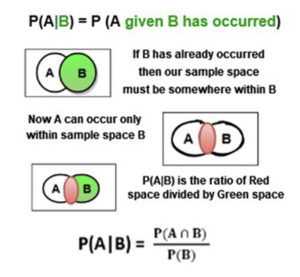
Conditional probability is defined as the likelihood of an event or outcome occurring, based on the occurrence of a previous event or outcome. It is the measure of the probability of an event A, given that another event B has already occurred.
When P(B) is not zero, then we can write the formula in the quotient form and visualize the conditional probability as a ratio.
Independent Events:
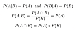
This is a special case of Conditional Probability, where the occurrence of one event does not affect the probability of another event. In other words, for two events A and B:
Bayes' Theorem Definition:
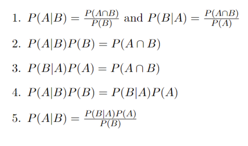
Bayes' Theorem Derivation: Starting with the definition of Conditional Probability
In Step 1 with the definition of conditional probabilities, it is assumed that P(A) and P(B) are not 0.
In Step 2 we multiply both sides by P(B) and in step 3 we multiply both sides by P(A) and we end up with the same result on the right hand side of each.
In Step 4 we are able to set both left sides equal to each other since they both have the same right hand side.
In Step 5 we divide both sides by P(B) and we arrive at Bayes' Theorem.
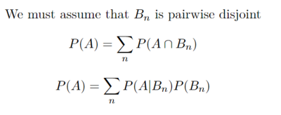
It is also important to introduce the law of total probability:
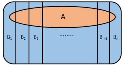
A picture depicting what is going on in this formula:
When applying these formulas with n = 2 we get:
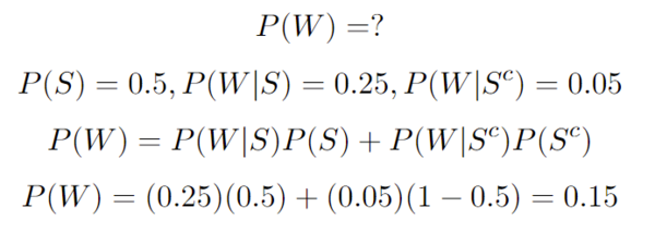
A quick example using the law of total probability: We can let P(W) be the probability that someone will wreck their car. Let P(S) be the probability that it will snow. Let’s say that the probability of wrecking is 0.05 with no snow and 0.25 with snow. We also know that there is a 0.5 chance of snow.
The law of total probability is commonly used in Bayes' rule. It is very useful, because it provides a way to calculate probabilities by using conditional and marginal probabilities. This is used commonly to compute the denominator when given partitions of the conditional probabilities. In many examples using Bayes' rule the probability P(B) in the denominator will be left and the law of total probability is generally the easiest way to solve for this. After solving for this it is easy to plug the values into Bayes' Theorem to get the value of P(A|B).
In the following example this direct application of the law of total probability will be used. When we combine the total probability with Bayes' Theorem we get the following equation which will be used in the next examples.
In this example we are able to solve for the probability of A by just using the probability of A given B, the probability of A given the complement of B, and the probability of B.
Bayes' Disease Example:
Say for example that you have tested positive for a disease which affects 0.1% of the population using a test which correctly identifies people who have the disease 99% of the time whilst also only incorrectly identifying people who do not have the disease 1% of the time, meaning that it has a false positive rate of 1%, and a true positive rate of 99%. What is the percent chance that you actually have this disease?
Intuitively, you might say that because the test has a success rate of 99%, then the chance that you actually have this disease is also 99%, but you would actually be incorrect.
In order to find the actual probability that you have this disease, we need to use Bayes' Theorem on our data. We want to know the probability of having the disease (D), given that we have tested positive (+), thus we want to find P(D|+). We know the probability of someone having the disease is 0.1%, P(D), we also know the probability of testing positive given that you have the disease is 99% P(+|D), and lastly, we know the probability of testing positive given that you don't have the disease is 1% P(+|D'). By plugging these values into the equation for Bayes' Rule, we can find the probability of having the disease given we tested positive:
Applying Bayes' Rule:
By applying the law of total probability, we get:
Lastly, by plugging in our values we get:
Our final result states that the probability of you actually having the disease if this test returns positive is only about 9%. This result may seem unintuitive, but will make much more sense when viewed from another perspective.
Say, for example, that you have a sample population of 1000 people, then given that the probability that 0.1% of people are affected by this disease, we can say that 1 person in this thousand are likely to have the disease:
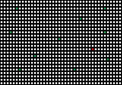
If everyone in this sample is given a test for the disease, then it is likely that we will have 10 people who test positive for this disease who do not have the disease (false positives, marked in green), and 1 person who tests positive and does have the disease (true positive, marked in red):
Then the person who actually has the disease and tests positive is only 1 among 11 people in the sample who tested positive.
Thus the probability that your test result is a true positive, is 1/11, or roughly 9%. This, obviously, is not a very conclusive or satisfactory result so what we can do to try and see if this positive result is accurate is to take another test.
Say that you take the exact same test again and it also returns positive. One thing we can do in Bayesian statistics is, upon receiving new information, we can update our prior probability with the probability we calculated previously, called the posterior probability. This is a very important part of Bayesian statistics as what we are doing is incorporating more/new evidence to improve our guess of the likelihood of an event occurring which can be extremely useful in predictive tasks where we can update our guess when new information is found (such as in machine learning). In our case we would like to improve our guess on the likelihood of you having this disease. To update our prior probability, we now know that the probability that we have the disease is 9%, so we replace the P(D) from our previous equation with P(D) = 0.09:
With this result, we know that it is likely that we have this rare disease but notice that this percentage is still below the 99% success rate of the test. This is simply one of many ways in which people can manipulate and misrepresent statistics. If people were to report that this test is successful 99% of the time, most people would automatically assume that they have the disease if the test returned positive when the chance is actually much lower. There are a lot of ways in which people can trick you with statistics if you aren’t armed with the knowledge to interpret and understand the nuances behind them. This is just one simple example of how seemingly simple statistics at face value, can have surprising and unintuitive meanings.
So how does this apply to the real world? For this we will look at data for COVID 19:
Using data from the CDC, we know that the total number of reported cases in the United States as of November 18, 2022 is 98,174,364 (https://www.cdc.gov/coronavirus/2019-ncov/covid-data/covidview/index.html, observed November 29, 2022). Using this value and dividing by the US population from the U.S. census as of November 27, 2022 (333,318,862), we can calculate that the prevalence of COVID-19 in the US is 98,174,364/333,318,862 = 0.29453587898 = 0.295% = P(D). For this example, we will look at the accuracy of the at home antigen tests. Taking data from a review of studies published by Cochrane, the authors found that in summary, antigen tests used on people who have symptoms showed a false positive rate of 11% P(+|D') and a false negative rate of 1% P(-|D), using this we can find the true positive rate with P(+|D) = 1 - 1% = 99% (https://www.cochrane.org/CD013705/INFECTN_how-accurate-are-rapid-antigen-tests-diagnosing-covid-19#:~:text=Using%20summary%20results%20for%20symptomatic,them%20really%20had%20COVID-19%3A&text=45%20people%20would%20test%20positive,19%20(false%20positive%20result), observed November 29, 2022). If someone with COVID symptoms were to use one of these tests and receive a positive result, we can plug in these values to Bayes' rule to find the probability that they actually have COVID:
We can see that the probability of the subject actually having COVID is only 79%, which is noticeably lower than the test's true positive rate of 99% and leaves a bit of uncertainty about whether or not the subject truly has COVID. We can again try to improve our guess by taking another test. In the case that it returns positive we see:
After two positive tests we can see that the probability of the subject actually having COVID-19 is now 97% with which we can more reasonably assume that this subject has COVID.
These results seem to be quite good for people who have symptoms but what about people who test without symptoms of COVID-19? Pulling data from the report by Cochrane once again, we have the false positive rate is 48% P(+|D'), and the false negative rate is 0.2% meaning our true positive rate is P(+|D) = 1 - .2% = 99.8%. Plugging into Bayes Theorem we get:
With a positive result, the subject has less than a 50% chance of actually having COVID, a stark difference from our symptomatic example, leaving a lot of room for doubt on whether or not this subject actually has COVID. What happens to this probability if we test positive a second time? By updating our prior probability we see that:
Our subject's chance of having COVID has only increased to 64%, which might be a surprisingly small increment given we have tested positive two times in row. This also means that we have 36% chance of this being two consecutive false positives which is pretty significant. What happens again if we get a third positive result?:
Our subject's probability of having COVID has now increased to 79%, which is high, but still leaves a 21% (over 1/5) chance of not actually having COVID, that means that there is reasonable chance that we have had 3 false positives in a row! How about if we finally get a fourth consecutive positive result?:
Our probability of the subject having COVID lands on 89% which is still leaves an 11% (~1/9) chance of of not having COVID. These results may be shocking, however, we also have to keep in mind that there are definitely some flaws with these calculations because our data isn't perfect. The value we used to estimate the prevalence of COVID-19 in the United States will very likely be inaccurate as not all cases of the disease are discovered and/or reported. We also can't know for certain that the values we used for success and failure rates of the test are accurate as the studies which the data was pulled from may have had flaws in their experimentation. Lastly, the accuracies of tests from different companies also vary and their success rate for different variants of COVID-19 vary as well so we should not treat these calculations as totally accurate but more of a rough estimate. What this should certainly highlight, however, is how easily statistics can be used deceptively. As we can see, the true positive rate of a test and the actual chance of a person having a disease should they test positive can be wildly different, which could be used to have people falsely believe that they have a certain disease without technically stating any falsehoods: "The test is accurate 99% of the time, so you probably have the disease". The results of these tests could also be used to inflate numbers for disease infection rates if each positive test is reported as a new case of a disease when in reality, the chances of a positive test being representative of an actual case of the disease could be very low (if we reported every non-symptomatic positive result as a new case, we might double the number of cases!). These are just some of the reasons why being armed with an understanding of statistics can be useful for understanding the actual implications of data.
Sources:
https://www.census.gov/popclock/
https://www.cdc.gov/coronavirus/2019-ncov/covid-data/covidview/index.html
Reference Book : A First Course in Probability, by Sheldon Ross, 9th edition or later

