(→Proving the Sampling Theorem) |
|||
| (8 intermediate revisions by the same user not shown) | |||
| Line 1: | Line 1: | ||
| − | + | == Proving the Sampling Theorem == | |
The sampling can be represented by "Impulse-train Sampling." | The sampling can be represented by "Impulse-train Sampling." | ||
| Line 9: | Line 9: | ||
We can recover <math>x(t)</math> from <math>x_p(t)</math> as follows: | We can recover <math>x(t)</math> from <math>x_p(t)</math> as follows: | ||
| − | <math>x_p(t) | + | <math>x_p(t) \rightarrow H(\omega) \rightarrow x_r(t)</math> |
| − | Where <math>H(omega)</math> is a filter with gain equal to the period of the signal and a cutoff frequency of <math>omega_c</math>. | + | Where <math>H(\omega)</math> is a filter with gain equal to the period of the signal and a cutoff frequency of <math>\omega_c</math>. |
| − | <math>omega_c | + | <math> \omega_c \rightarrow \omega_m < \omega_c < \omega_s - \omega_m</math>. |
| + | |||
| + | This process can be easily shown in the frequency domain graphically. An example is below. | ||
| + | |||
| + | [[Image:Freq_Domain_ECE301Fall2008mboutin.jpg|Graph]] | ||
Latest revision as of 19:44, 10 November 2008
Proving the Sampling Theorem
The sampling can be represented by "Impulse-train Sampling."
$ x_p(t) = ? $ $ x_p(t) = x(t)p(t) $ $ x_p(t) = x(t)\sum_{n=-\infty}^{\infty} \delta(t-nT) $
We can recover $ x(t) $ from $ x_p(t) $ as follows:
$ x_p(t) \rightarrow H(\omega) \rightarrow x_r(t) $
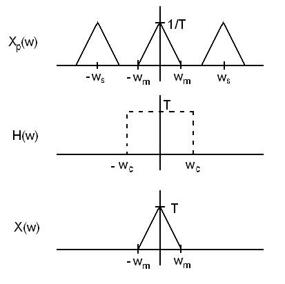
Where $ H(\omega) $ is a filter with gain equal to the period of the signal and a cutoff frequency of $ \omega_c $.
$ \omega_c \rightarrow \omega_m < \omega_c < \omega_s - \omega_m $.
This process can be easily shown in the frequency domain graphically. An example is below.


