(New page: Category:bonus point project Category:ECE302 Category:probability <center><font size= 4> '''Correlation vs Covariance''' </font size> Student project for ECE302 by Blue ...) |
|||
| (21 intermediate revisions by 2 users not shown) | |||
| Line 13: | Line 13: | ||
---- | ---- | ||
---- | ---- | ||
| − | == | + | ==Introduction== |
| − | + | ||
| − | + | I was taking ECE 302, a course on probability, random variables, and random processes, when all of a sudden I got overwhelmed with all of these different statistical numbers describing relations of datasets or random variables. So, I decided to crack down on some research and bring the important ideas all in one spot so that future students (or anyone for that matter) can quickly understand the differences between these functions. Feel free to comment and ask questions | |
| − | + | ||
| − | + | ---- | |
| − | + | ||
| − | == | + | ==Definitions== |
| − | + | Source: Dictionary.com | |
| + | |||
| + | '''Variation:''' This is used to analyze the spread of the data being observed. | ||
| + | |||
| + | '''Standard Deviation:''' This is a measure of how spread out a set of numeric values is about its mean. | ||
| + | |||
| + | '''Covariance:''' This is a measure of two random variable’s association with each other. | ||
| + | |||
| + | '''Correlation:''' This is the degree to which two random variables vary with each other. | ||
| + | |||
| + | '''Autocovariance:''' This is the measure of two data points of a random variable’s association with each other | ||
| + | |||
| + | '''Autocorrelation:''' This is the degree to which two data points of a random variable vary with each other | ||
| + | |||
| + | Notice the similarity between variation and standard deviation, covariance and correlation, covariance and autocovariance, and correlation and autocorrelation. | ||
---- | ---- | ||
| + | |||
| + | ==Mathematical Definitions== | ||
| + | Source: Professor Pollak's Random Signals Lecture Notes | ||
| + | |||
| + | '''Variation:''' | ||
| + | |||
| + | <math> | ||
| + | Var(X) = E[(X-\mu)(X-\mu)] = E[(X-\mu)^{2}] | ||
| + | </math> | ||
| + | |||
| + | Looking ahead, the variance of X, Var(X) can also be described as the covariance of X with X, Cov(X,X). If you go to the covariance definition and use the variable X instead of Y, you will obtain the definition of variance. Another popular way of defining variance is | ||
| + | |||
| + | <math> | ||
| + | Var(X) = E[X^{2}] - (E[X])^{2} | ||
| + | </math> | ||
| + | |||
| + | This is derived by manipulating the definition above using the rules | ||
| + | of expected value. | ||
| + | |||
| + | '''Standard Deviation:''' | ||
| + | |||
| + | <math> | ||
| + | \sigma = \sqrt{E[(X-\mu)^{2}]} = \sqrt{Var(X)} | ||
| + | </math> | ||
| + | |||
| + | The standard deviation is simply the square root of the variance. | ||
| + | |||
| + | '''Covariance:''' | ||
| + | |||
| + | <math> | ||
| + | \sigma(X,Y) = E[(X-\mu_{x})(Y-\mu_{y})] | ||
| + | </math> | ||
| + | |||
| + | Remember that the covariance is a relation of two random variables, X and Y. As it was mentioned previously, if you find the covariance of X and X, you will simply obtain the variance of X | ||
| + | |||
| + | '''Correlation:''' | ||
| + | |||
| + | <math> | ||
| + | \rho_{X,Y} = \frac{cov(X,Y)}{\sigma_{X}\sigma_{Y}} = \frac{E[(X-\mu_{X})(Y-\mu_{Y})]}{\sigma_{X}\sigma_{Y}} | ||
| + | </math> | ||
| + | |||
| + | This puts the covariance on terms that is more understandable and quickly comparable. An example of this will be shown more clearly in the walkthrough. | ||
| + | |||
| + | '''Autocovariance:''' | ||
| + | |||
| + | <math> | ||
| + | \sigma_{X_{1}X_{2}}(n1,n2) = E[(X_{1}-\mu_{n1})(X_{2}-\mu_{n2})] | ||
| + | </math> | ||
| + | |||
| + | The autocovariance is just like the formula for covariance but instead of finding the relation of two random variables, you are finding the relation of two data points from one random variable. | ||
| + | |||
| + | '''Autocorrelation:''' | ||
| + | |||
| + | <math> | ||
| + | \rho_{X_{1},X_{2}} = \frac{cov(X_{1},X_{2})}{\sigma_{X_{1}}\sigma_{X_{2}}} = \frac{E[(X_{1}-\mu_{X_{1}})(X_{2}-\mu_{X_{2}})]}{\sigma_{X_{1}}\sigma_{X_{2}}} | ||
| + | </math> | ||
| + | |||
| + | This is like the correlation formula except it also finds the relation of two data points from one random variable instead of finding the relation of two random variables. | ||
| + | |||
| + | ---- | ||
| + | |||
| + | ==Walkthrough== | ||
| + | |||
| + | To start off, I will walk through the calculations of variation and standard deviation on a sample data set: | ||
| + | |||
| + | [[Image:Table1.png]] | ||
| + | |||
| + | Firstly, to find the variance of X,find the mean, <math>\mu</math>. Just (1+2+3+4+5+6+7) / 7 = 4. Just as the formula for variation states, take all of the X values and subtract the mean, giving you this new data: | ||
| + | |||
| + | [[Image:Table2.png]] | ||
| + | |||
| + | And now square the data in the right row: | ||
| + | |||
| + | [[Image:Table3.png]] | ||
| + | |||
| + | Finally, take the expected value or the mean of this new column, just as is shown in the formula. The mean of the column is 4. Thus the variance of this variable X is 4. To find the standard deviation, simply take the square root of the variance. In this case the square root of 4, which is 2. | ||
| + | |||
| + | Now do the exact same process, however for another variable Y. This so that you can start examining the covariance and correlation. | ||
| + | |||
| + | [[Image:Table5.png]] | ||
| + | |||
| + | Now that you have two variables, X and Y, you can find the relations between them. As stated in the formula you need (X-\mu_{x})(Y-\mu_{y}). Now all you need to do is multiply columns 3 and 4 together. | ||
| + | |||
| + | [[Image:Table4.png]] | ||
| + | |||
| + | To find the covariance, you need to find the expected value, or the mean, of the last column, just as is stated in the formula. Doing so, you get 4. What does 4 really mean though, do X and Y change together perfectly? Do they not? From the covariance it is quite difficult to determine this. Thus, we calculate the correlation which has a range of -1 to 1, where 1 is perfectly correlated and -1 is perfectly correlated in the inverse direction. The correlation can be calculated quickly as the covariance over the standard deviations multiplied. For this example, there is a correlation of 1. This tells you that the set is perfectly correlated, and you can see that this is true because as X increases Y also increases the exact same way. | ||
| + | |||
| + | If X and Y are independent of each other, that means they are uncorrelated with each other, or cov(X,Y) = 0. However, if X and Y are uncorrelated, that does not mean they are independent of each other. 1, -1, and 0 are the three extreme points <math>\rho X,Y)</math> can represent. [1] | ||
| + | |||
| + | ---- | ||
| + | |||
| + | ===Examples=== | ||
| + | The following are examples from Professor Pollak's General Random Variables lecture notes of what real data may look like: | ||
| + | |||
| + | [[Image:correlation_coefficient_graph_pxy0.png|300px]] | ||
| + | |||
| + | This an example of a data set when the correlation is 0 | ||
| + | |||
| + | [[Image:correlation_coefficient_graph_pxy10.png|300px]] | ||
| + | |||
| + | This an example of a data set when the correlation is 1 | ||
| + | |||
| + | [[Image:correlation_coefficient_graph_pxy-10.png|100px]] | ||
| + | |||
| + | This an example of a data set when the correlation is -1 | ||
| + | |||
| + | [[Image:correlation_coefficient_graph_pxy0_2.png|100px]] | ||
| + | |||
| + | This an example of a data set when the correlation is .2 | ||
| + | |||
| + | [[Image:correlation_coefficient_graph_pxy4.png|300px]] | ||
| + | |||
| + | This an example of a data set when the correlation is .4 | ||
| + | |||
| + | [[Image:correlation_coefficient_graph_pxy-7.png|250px]] | ||
| + | |||
| + | This an example of a data set when the correlation is -.7 | ||
| + | |||
| + | [[Image:correlation_coefficient_graph_pxy9.png|200px]] | ||
| + | |||
| + | This an example of a data set when the correlation is .9 | ||
| + | |||
| + | ---- | ||
| + | |||
| + | ==Questions/Comments/Concerns:== | ||
| + | * | ||
| + | * | ||
| + | * | ||
| + | ---- | ||
| + | ==References== | ||
| + | [1]: Ilya Pollak. General Random Variables. 2012. Retrieved from https://engineering.purdue.edu/~ipollak/ece302/SPRING12/notes/19_GeneralRVs-4_Multiple_RVs.pdf | ||
| + | |||
| + | [2]: Ilya Pollak. Random Signals. 2004. Retrieved from https://engineering.purdue.edu/~ipollak/ee438/FALL04/notes/Section2.1.pdf | ||
| + | |||
| + | [3]: Dictionary.com Retrieved from https://www.dictionary.com | ||
| + | |||
[[2013_Spring_ECE_302_Boutin|Back to ECE302 Spring 2013, Prof. Boutin]] | [[2013_Spring_ECE_302_Boutin|Back to ECE302 Spring 2013, Prof. Boutin]] | ||
Latest revision as of 06:19, 5 May 2013
Correlation vs Covariance
Student project for ECE302
by Blue
Contents
Introduction
I was taking ECE 302, a course on probability, random variables, and random processes, when all of a sudden I got overwhelmed with all of these different statistical numbers describing relations of datasets or random variables. So, I decided to crack down on some research and bring the important ideas all in one spot so that future students (or anyone for that matter) can quickly understand the differences between these functions. Feel free to comment and ask questions
Definitions
Source: Dictionary.com
Variation: This is used to analyze the spread of the data being observed.
Standard Deviation: This is a measure of how spread out a set of numeric values is about its mean.
Covariance: This is a measure of two random variable’s association with each other.
Correlation: This is the degree to which two random variables vary with each other.
Autocovariance: This is the measure of two data points of a random variable’s association with each other
Autocorrelation: This is the degree to which two data points of a random variable vary with each other
Notice the similarity between variation and standard deviation, covariance and correlation, covariance and autocovariance, and correlation and autocorrelation.
Mathematical Definitions
Source: Professor Pollak's Random Signals Lecture Notes
Variation:
$ Var(X) = E[(X-\mu)(X-\mu)] = E[(X-\mu)^{2}] $
Looking ahead, the variance of X, Var(X) can also be described as the covariance of X with X, Cov(X,X). If you go to the covariance definition and use the variable X instead of Y, you will obtain the definition of variance. Another popular way of defining variance is
$ Var(X) = E[X^{2}] - (E[X])^{2} $
This is derived by manipulating the definition above using the rules of expected value.
Standard Deviation:
$ \sigma = \sqrt{E[(X-\mu)^{2}]} = \sqrt{Var(X)} $
The standard deviation is simply the square root of the variance.
Covariance:
$ \sigma(X,Y) = E[(X-\mu_{x})(Y-\mu_{y})] $
Remember that the covariance is a relation of two random variables, X and Y. As it was mentioned previously, if you find the covariance of X and X, you will simply obtain the variance of X
Correlation:
$ \rho_{X,Y} = \frac{cov(X,Y)}{\sigma_{X}\sigma_{Y}} = \frac{E[(X-\mu_{X})(Y-\mu_{Y})]}{\sigma_{X}\sigma_{Y}} $
This puts the covariance on terms that is more understandable and quickly comparable. An example of this will be shown more clearly in the walkthrough.
Autocovariance:
$ \sigma_{X_{1}X_{2}}(n1,n2) = E[(X_{1}-\mu_{n1})(X_{2}-\mu_{n2})] $
The autocovariance is just like the formula for covariance but instead of finding the relation of two random variables, you are finding the relation of two data points from one random variable.
Autocorrelation:
$ \rho_{X_{1},X_{2}} = \frac{cov(X_{1},X_{2})}{\sigma_{X_{1}}\sigma_{X_{2}}} = \frac{E[(X_{1}-\mu_{X_{1}})(X_{2}-\mu_{X_{2}})]}{\sigma_{X_{1}}\sigma_{X_{2}}} $
This is like the correlation formula except it also finds the relation of two data points from one random variable instead of finding the relation of two random variables.
Walkthrough
To start off, I will walk through the calculations of variation and standard deviation on a sample data set:
Firstly, to find the variance of X,find the mean, $ \mu $. Just (1+2+3+4+5+6+7) / 7 = 4. Just as the formula for variation states, take all of the X values and subtract the mean, giving you this new data:
And now square the data in the right row:
Finally, take the expected value or the mean of this new column, just as is shown in the formula. The mean of the column is 4. Thus the variance of this variable X is 4. To find the standard deviation, simply take the square root of the variance. In this case the square root of 4, which is 2.
Now do the exact same process, however for another variable Y. This so that you can start examining the covariance and correlation.
Now that you have two variables, X and Y, you can find the relations between them. As stated in the formula you need (X-\mu_{x})(Y-\mu_{y}). Now all you need to do is multiply columns 3 and 4 together.
To find the covariance, you need to find the expected value, or the mean, of the last column, just as is stated in the formula. Doing so, you get 4. What does 4 really mean though, do X and Y change together perfectly? Do they not? From the covariance it is quite difficult to determine this. Thus, we calculate the correlation which has a range of -1 to 1, where 1 is perfectly correlated and -1 is perfectly correlated in the inverse direction. The correlation can be calculated quickly as the covariance over the standard deviations multiplied. For this example, there is a correlation of 1. This tells you that the set is perfectly correlated, and you can see that this is true because as X increases Y also increases the exact same way.
If X and Y are independent of each other, that means they are uncorrelated with each other, or cov(X,Y) = 0. However, if X and Y are uncorrelated, that does not mean they are independent of each other. 1, -1, and 0 are the three extreme points $ \rho X,Y) $ can represent. [1]
Examples
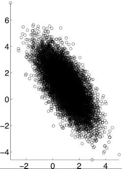
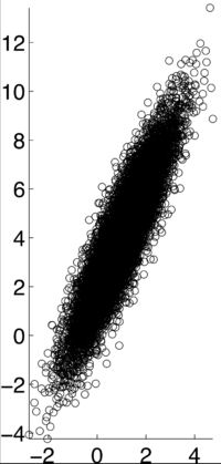
The following are examples from Professor Pollak's General Random Variables lecture notes of what real data may look like:
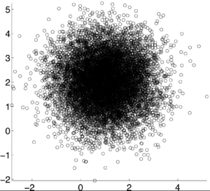
This an example of a data set when the correlation is 0
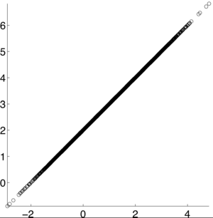
This an example of a data set when the correlation is 1
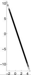
This an example of a data set when the correlation is -1
This an example of a data set when the correlation is .2
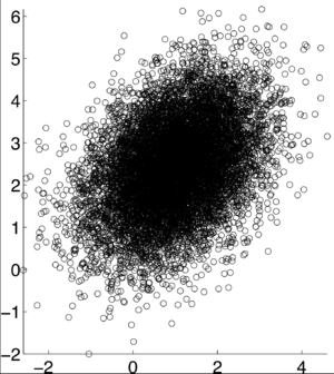
This an example of a data set when the correlation is .4
This an example of a data set when the correlation is -.7
This an example of a data set when the correlation is .9
Questions/Comments/Concerns:
References
[1]: Ilya Pollak. General Random Variables. 2012. Retrieved from https://engineering.purdue.edu/~ipollak/ece302/SPRING12/notes/19_GeneralRVs-4_Multiple_RVs.pdf
[2]: Ilya Pollak. Random Signals. 2004. Retrieved from https://engineering.purdue.edu/~ipollak/ee438/FALL04/notes/Section2.1.pdf
[3]: Dictionary.com Retrieved from https://www.dictionary.com


