Object Tracking Using Matlab

An ECE438 project by Matt Miller.

In the high tech world we live in, the number of applications which require image processing is growing rapidly. Improvements in computer technology have resulted in even small portable devices such as cellular phones becoming powerful enough to support image processing in real time, and people all around the world are coming up with amazing real-life applications for this technology. This project is a small experiment to show how simple it can be to write an object tracking script in Matlab without relying entirely on the advanced features of Matlab's Image Processing Toolbox or Computer Vision Toolbox, such as the built in Kalman Filter function.

Let's begin by opening up Matlab and plugging in a webcam. While a previously recorded video can be used, it is definitely a lot more interesting to capture your own, and it can be very beneficial to use this as a chance to learn how to set up a camera with Matlab for image processing, even though we will not be doing any calculations in real time. 

webcam = videoinput('winvideo', 1, 'RGB24_640x480');
set(webcam, 'FramesPerTrigger', 120);
set(getselectedsource(webcam), 'FrameRate', '30')
set(getselectedsource(webcam), 'WhiteBalanceMode', 'manual')

Here we see an example of the code needed to initialize a USB webcam in Matlab, where "winvideo" is the device type, "1" is the device number, and "RGB24_640x480" is the device mode being used, which stands for a 640x480 24bpp RGB image. In the next line, we can set the "FramesPerTrigger" value for "webcam", which is the total number of frames we would like the camera to capture in one trigger. Then we move on to setting the frame rate, which is best set to the maximum supported rate. If a lower framerate is desired, it is best to record the video at the highest frame rate and then decimate, as lowering the frame rate usually lowers the refresh rate of the image sensor, which can cause significant amounts of motion blur in the video. Next, we set the white balance to manual, as we want the camera to make as few corrections as possible while filming, as doing so will cause problems when attempting to obtain the difference of frames.

Now let's start recording:

start(webcam)
preview(webcam)
wait(webcam)
rawvideo = getdata(webcam);
closepreview

In this block of code, we trigger the webcam with the start function, and then open a preview window to see what's filming in real time. I have chosen to tell Matlab to wait for the camera to finish before moving on, however if I wished to perform image processing in real time I would omit this line and the script would continue to run while more frames are added to the video. Once the webcam has captured the preset number of frames, the video is stored as a 4-D matrix with the paramters height, width, color, and frame.

Now that we have a video, we need to convert it to grayscale in order to start the processing. In more complex vision systems, this step is not done, and the processing takes the color values into effect. Since we are only doing simple object tracking, a simple 2-D matrix is all that is needed. In this code, we can also decimate the video input. When determining the ideal input settings, you want to take into account the size of the object and the speed it will travel at. If the object is large and/or not moving very fast, the object will have a large overlap in each frame. Depending on the surface details of the object, this may cause the detection program to only pick up the leading and trailing edges of the object. To prevent this, we can decrease the frame rate of the input so that the change in location falls between the minimum change needed for detection and the length of the object in the direction of travel. In this range, the change will be great enough, but it will not be too large to that the path is averaged. As mentioned earlier, simply decreasing the capture rate of the camera will decrease the refresh rate of the image sensor, so instead we can film at the maximum frame rate and drop frames, or decimate the video:

[H,W,C,F] = size(rawvideo);
for f = (F/N):-1:1
    gvid(:,:,f) = rgb2gray(rawvideo(:,:,:,N*f));
end
s = size(gvid);

In this code, the term N is the decimation factor. If N is set as 1, every frame will be used, and if N is set as 2, every other frame will be used.

At this point, we can also filter the video if it is too noisy of choppy. First, we can get rid of noise with a Gaussian filter:

gvids = gvid;
for r = s(3):-1:1
    gvids(:,:,r) = uint8(filter2(gaussFilter(9,1),gvid(:,:,r)));
end

The filter shown here is a NxN(in this case 9x9) Gaussian filter generated using the "gaussFilter" built during lab. The Gaussian filter built into the filter2 function can alternatively be used.
If needed, we can also try averaging frames, although doing so may make differencing difficult. In this example, a frame is weighted by 2:3 the current frame and 1:3 the next frame:

gvids2 = gvids;
for g = s(3)-1:-1:2
    gvids2(:,:,g) = (gvids(:,:,g) + 0.5*gvids(:,:,g+1))/1.5;
end

Next, we move on to one of the most important steps: the differencing of the frames using the imabsdiff function:

dtvid = zeros(s);
for a = s(3)-1:-1:1
    diffvid(:,:,a) = imabsdiff(gvids(:,:,a),gvids(:,:,a+1));
    gt(a) = graythresh(diffvid(:,:,a));
    if gt(a) > 0.01
        dtvid(:,:,a) = (diffvid(:,:,a) >= (gt(a) * 255));
    else
        dtvid(:,:,a) = 0;
    end
end

For each frame, a difference frame is generated by subtracting the following frame to obtain the absolute difference. These frames can be very difficult to use, so code is added to the loop to quantize the image to binary values. The function graythresh returns a threshold value between 0 and 1, which is then compared pixel-by-pixel. If the pixel is above 255 time the threshold value, it is set to 1, and all values below are left at 0. The resulting output is a matrix of type logical, however most Matlab imaging commands will correctly interpret it as a grayscale image, and it can be converted to a different scale using uint8 or double.

Next, we will remove all small objects with the bwareaopen function. This function removes all objects in a binary image under a specified size, and optionally using a specified connectivity:

for g = s(3):-1:1
    dtvid2(:,:,g) = bwareaopen(dtvid(:,:,g), 20,8);
end

In this example, all objects with an area less than 20 are converted to zeros, and the two-dimensional eight-connected neighborhood is used.

Now we should have a black image with only two white objects: where the moving object currently is in relation to the previous frame, and where the object no longer is in relation to the first frame. If the object is not moving very fast in relation to the frame rate, and the surface looks fairly uniform, the highlighted areas will be the leading and trailing edges of the object, with the center remaining black. The next step is to identify the centroid of the object, but since we have two objects we will need to select one. In order to do this, we will use the regionprops function to obtain the centroid and area of each object in the frame:

centroids = zeros(s(3),2);
for n = 1:1:s(3)
    if sum(sum(dtvid2(:,:,n))) > 0
        reg = regionprops(logical(dtvid2(:,:,n)),'area', 'centroid');
        av = [reg.Area];
        [value, index] = max(av);
        centroids(n,:) = reg(index(1)).Centroid;
    end
end

Once these parameters are obtained, they are then stored in a matrix from largest to smallest. The centroid coordinate for the first entry, which represents the object with the largest area, is then chosen and stored in the centroids matrix.

Small changes in lighting and other noise may have still made it through the filtering at this point, so let's apply a filter to the centroids matrix that filters out any sets of centroids that do not appear in at least 5 consecutive frames:

for p = 3:1:s(3)-2
    if centroids(p-2,1) && centroids(p+2,1) == 0
        centroids(p,1) = 0;
    end
    if centroids(p-2,2) && centroids(p+2,2) == 0
        centroids(p,2) = 0;
    end
end

Now we have identified the moving object in each frame and a centroid-based estimation of the location in each frame. The next step is to display the data. First we plot the last frame of the raw color video:

clear figure(1)
figure(1)
imshow(rawvideo(:,:,:,s(3)))
hold on

Now that we have drawn a frame, let's superimpose the centroids on top:

for j = 1:1:s(3)
    if centroids(j,1) && centroids(j,2) > 0
        plot(centroids(j,1),centroids(j,2),'ro')
        hold on
    end
end

Next, we would like to connect the points. This however raises a problem, as any time a centroid is not located, the previous location is connected to (0,0), along with the first and last values. To fix this, we will need to change each (0,0) value to NaN so that the zero values are not shown, and then plot the data:

q = centroids(:,1);
q(~q) = NaN;
v = centroids(:,2);
v(~v) = NaN;
plot(q,v,'r')

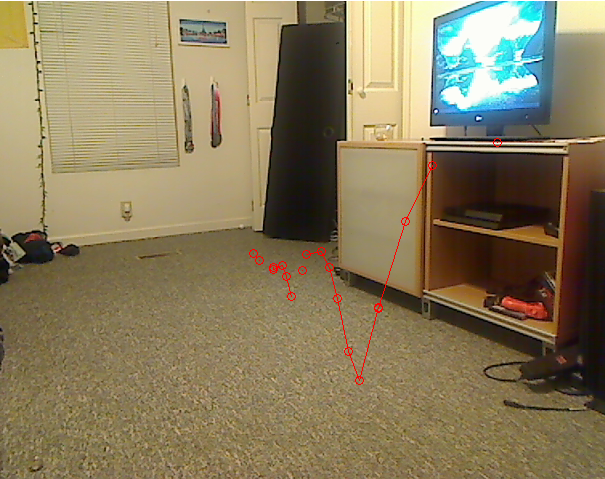
Now let's take a look at an example result of a bouncing ball:

 
Notice the where the dots are not connected, these are locations where the program "loses track" of the ball".
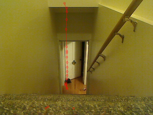
In this example, a bag has been thrown down a set of stairs. Notice the incorrect locations, these are generally picked up in the first few frames and make it through the filtering. In my tests, I found that the pattern on the carpet, which resembles noise, is generally to blame.
 

Works Cited:
Lee, Dan, and Steve Eddins. "Tracking Objects: Acquiring And Analyzing Image Sequences In MATLAB."

   Tracking Objects: Acquiring And Analyzing Image Sequences In MATLAB. MathWorks, 2003. Web. 05 Dec. 2013.

Back to 2013 Fall ECE 438 Boutin