Hidden Markov Chains

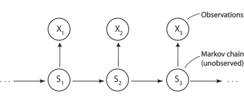
The idea of the hidden Markov chain was raised by an American mathematician Leonard Baum and his colleagues in the 1960s. The hidden Markov chain is an extension of the Markov chain: compared to the traditional Markov chain, the state $ S_{t} $ of the hidden Markov chain at certain time step $ t $ can not be observed; however, at every time step $ t $, there is an output state $ X_{t} $ and the observable output state $ X_{t} $ only relates to the unobservable state $ S_{t} $. A typical hidden Markov chain model can therefore be illustrated as follows:

Diagram courtesy of Jan Bulla

To get a better understanding of the hidden Markov chain model, let’s use the weather example again. However, we have to make some variations for this time. Now, assume your friend is living in another country. He tells you what he has done everyday (Assume he only does one thing a day, and his behavior is only related to the weather of that particular day). Now, you are trying to predict the weather in his country based on the information he tells you for a particular time span. In this case, the weather we are trying to predict during these days is called the state sequence (correspond to $ S_{1}, S_{2}, S_{3}, ... $ in the diagram above), and a series of behavior your friend has conducted during these days is called the observation sequence (correspond to $ X_{1}, X_{2}, X_{3}, ... $ in the diagram above).

Such a weather-behavior hidden Markov chain model consists of five parts：

1. A set of Hidden States $ S: {S_{1}, S_{2}, ... S_{n}} $
2. A sequence of observations $ X: {X_{1}, X_{2}, ... X_{n}} $
3. The transition probability matrix $ A $ of Hidden States, representing the probability of moving from state $ S_{i} $ to $ S_{i+1} $
4. The transition probability matrix $ B $, also known as the emission probabilities; each expressing the probability of an observation $ X_{i} $ being generated from state $ S_{i} $.
5. The initial probability distribution over states $ P_{i} $

As Adam Smith once said: “you can't always get what you want.” Ideally, we know all five components; in reality, we only know some of them, and the goal is to use the given components to solve for the unknown ones. There are mainly three fundamental problems:

1. Given a Hidden Markov chain (A,B,P) and an observation sequence X, calculate the occurrence probability of that specific observation sequence.
2. Given a Hidden Markov chain (A,B,P) and an observation sequence X, find out the best hidden state sequence S.
3. We only know an observation sequence O and the set of states in the hidden Markov chain; we want to learn the components A and B of that hidden Markov chain.

The first problem is essentially a “predicting” problem. We can use forward and backward algorithms to solve it. The second problem is essentially a “decoding” problem. We can use the Viterbi algorithms to solve problems of this type. The third problem is essentially a machine learning problem, and the Baum-Welch Algorithm is used most frequently.

Back to Markov Chains