Filtering Text On A Chalkboard
One of the issues with writing on a chalkboard is that chalk dust quickly accumulates. Eventually, even the eraser leaves more dust than it erases. For students in large classrooms or for those learning through online lectures, this can become a major issue, as words, equations, and calculations become hardly visible. The goal of this mini-project was to apply a low pass filter learnt in class and observe its effectiveness in removing the excess chalk dust (‘noise’) from the blackboard.
First, let’s look at the system we are trying to analyze. The background is a dark green chalkboard. The information that we want are the latest lines drawn by the chalk (we are assuming this chalk is the most white and intense part of the system, noting that this assumption does not always hold). The ‘noise’ here is the dust, or residual chalk marks, left behind from previous content that was erased. Our goal is to keep the sharp lines of chalk against the dark background, and remove only the extra chalk dust.
The reason for selecting a low pass filter is two-fold. Firstly, it is one of the simpler (and popular) filters to implement at this scale. Secondly, the low-pass filter is versatile enough to extend applications to any writing on a background, not just chalk against a chalkboard. It can be implemented for any image with text and noise.
Traditionally, low pass filters have been used on images taken in space to smoothen out noise from sharp light sources. They are also very popular in beauty enhancement features on Adobe Photoshop and in smartphones, to remove blemishes from portraits. You might be wondering: what does high frequency mean when filtering an image? Simply, it’s the more intense/bright parts of an image.
Below is the MATLAB code to implement a simple low-pass filter (LPF) on an image. It works by taking a window of pixels in the image and finding the average value for each of the three pixel colors: red, green, and blue (RGB) within the window. The program then replaces the center pixel value in this window with the averaged value. It repeats this process for all windows in the image. The expected result is that the image is slightly blurred, as the LPF’s purpose is to reduce the weight/minimize high frequency noise. The program was created from scratch, and thus not optimized. Its complexity is on the order of O(n4).
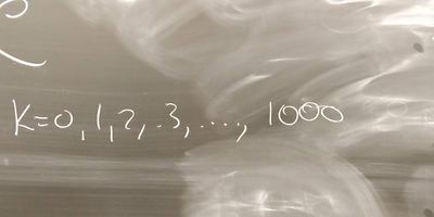
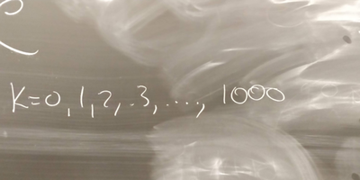
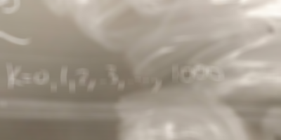
Below, you can see the results of the low pass filter on an image taken from Prof. Mimi’s classroom chalkboard. Three different window sizes were used, and one can see that the greater the window size, the greater the blurriness.
While this idea has been interesting to understand an explore, one can see that the result of the LPF is exactly the opposite of what we were looking for. Instead of sharpening the text, the program made it blurrier (this is more apparent with larger window sizes). The effect of the noise also decreases, but this is outweighed by the loss of clarity in the content. Part of the problem is that the noise is mostly at the low-frequency level, meaning that an LPF would not help much. From my discussion with Prof. Mimi, we discussed that to truly enhance the meaningful information on the chalkboard, we would need to have an ‘edge-detection’ program that essentially functions as a high-pass filter (HPF), to highlight the lines of the equations/letters/numbers. Then, by superimposing the HPF and LPF programs, a true ‘clarity-enhancer’ could be obtained.
Finally, an interesting question that came up was how this program might work in real time. From my limited knowledge, the answer is that while the program can be more optimized, it cannot be instantaneous. However, if people are watching through a video, this is not really an issue, as the latency can be built-in.
% Praneeth Medepalli
% ECE 301: Image Low Pass Filter
% April 1, 2019

% Extract the individual red, green, and blue color values as matrices
imData = imread('test1.jpg');
R = imData(:,:,1);
G = imData(:,:,2);
B = imData(:,:,3);

% Obtain dimensions of image in # of pixels
[picHeight,picLength] = size(R);

% Create new matrices for filtered image
Rnew = zeros(picHeight,picLength);
Gnew = zeros(picHeight,picLength);
Bnew = zeros(picHeight,picLength);

% Initialize pixel value counters
numPix = 0;
pixval = 0;

% Square window length - 1 (# of pixels)
windowSize = 2;
windowSize = windowSize / 2;

% Iterate over every pixel
for r = 1:picHeight
    for c = 1:picLength

        % Initialize pixel value counters
        numPix = 0;
        pixvalR = 0;
        pixvalG = 0;
        pixvalB = 0;
        newPixelR = 0;
        newPixelG = 0;
        newPixelB = 0;

        % Assign bounds of window to iterate over
        leftCol = c - windowSize;
        rightCol = c + windowSize;
        topRow = r - windowSize;
        botRow = r + windowSize;


        % Check for edge cases (out of bounds)
        if leftCol < 1
            leftCol = 1;
        end

        if rightCol > picLength
            rightCol = picLength;
        end

        if topRow < 1
            topRow = 1;
        end

        if botRow > picHeight
            botRow = picHeight;
        end

        % Iterate over window to find average pixel value
        for row = topRow:botRow
            for col = leftCol:rightCol
                pixvalR = pixvalR + double(R(row,col));
                pixvalG = pixvalG + double(G(row,col));
                pixvalB = pixvalB + double(B(row,col));
                numPix = numPix + 1;
            end
        end

        % Find average
        newPixelR = pixvalR / numPix;
        newPixelG = pixvalG / numPix;
        newPixelB = pixvalB / numPix;

        % Assign to new matrices
        Rnew(r,c) = uint8(newPixelR);
        Gnew(r,c) = uint8(newPixelG);
        Bnew(r,c) = uint8(newPixelB);
    end
end

% Recombine separate color matrices into an RGB image.
imRecons = cat(3, Rnew, Gnew, Bnew);

% Test to make sure original and reconstructed image are identical
%imshow(imRecons);
imData(:,:,1) = Rnew;
imData(:,:,2) = Gnew;
imData(:,:,3) = Bnew;

% Write data to file and compare to original picture
imwrite(imData,'testWindow2.png');
isequal(imData,imRecons)
Sources:
Frequency Filter. (2003). Retrieved March 30, 2019, from https://homepages.inf.ed.ac.uk/rbf/HIPR2/freqfilt.htm
Boutin, M. (2019, April 3). Personal interview.


