ECE600 F13 Stochastic Processes mhossain - Rhea

Back to all ECE 600 notes

Stochastic Processes

We have already seen discrete-time random processes, but we will now formalize the concept of random process, including both discrete-time and continuous time.

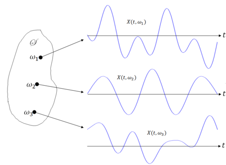
'Definition $ \qquad $ a stochastic process, or random process, defined on (S,F,P) is a family of random variables {X(t), t ∈ T} indexed by a set T.

Fig 1: The mapping from the sample space to the reals under X$ _j $.

Each waveform is referred to as a sample realization. Note that T can be uncountable, as shown above, or countable.

Note that

• X(t,$ \omega $) (or simply X(t)) is a random process.
• X(t$ _0 $,$ \omega $) is a random variable for fixed t$ _0 $.
• X(t,$ \omega_0 $) is a real-valued function of t for fixed $ \omega_0 $.
• X(t$ _0 $,$ \omega_0 $) is a real number for fixed t$ _0 $ and $ \omega_0 $.

There are four types or random processes we will consider

1. T ⊂ R uncountable, X(t) a discrete random variable for every t ∈ T is a continuous-time discrete random process.
2. T ⊂ R uncountable, X(t) a continuous random variable for every t ∈ T is a continuous time continuous random process.
3. T ⊂ R countable, X(t) a discrete random variable for every t ∈ T is a discrete-time discrete random process.
4. T ⊂ R countable, X(t) a continuous random variable for every t ∈ T is a discrete-time continuous random process.

Example $ \qquad $ if T = N = {1,2,3,...}, then X(t) is a discrete time random process, usually written as X$ _1 $,X$ _2 $

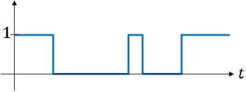
Example $ \qquad $ a binary waveform with random transition times

Fig 2: A binary waveform with random transition times.

Example $ \qquad $ A sinusoid with random frequency

where $ \Omega $ is a random variable.

Probabilistic Description of a Random Process

We can use joint pdfs of pmfs, but often we use the first and second order moments instead.

Definition $ \qquad $ The nth order cdf of X(t) is

and the nth order pdf is

Notation $ \qquad $ for n=1, we have

and for n= 2,

Definition $ \qquad $ The nth order pmf of a discrete random process is

It can be shown that if f$ _{X(t1)...X(tn)} $(x$ _1 $,...x$ _n $) is specified ∀t$ _1 $,...,t$ _n $; ∀n = 1,2,..., then X(t) is a valid random process consistent with a probability space (S,F,P). This result comes from the Kolmogorov existence theorem, which we will not cover.

Now consider the first and second order moments for a random process.

Definition $ \qquad $ The mean of a random process X(t) is

Definition $ \qquad $ The autocorrelation function of a random process X(t) is

Note: R$ _{XX} $(t$ _1 $,t$ _2 $) = R$ _{XX} $(t$ _2 $,t$ _1 $)

Definition $ \qquad $ The autocovariance function of a random process X(t) is

Important property of R$ _{XX} $ and C$ _{XX} $:
R$ _{XX} $ and C$ _{XX} $ are non-negative definite functions, i.e., ∀a$ _1 $,...,a$ _n $ ∈ R and t$ _1 $,...,t$ _n $ ∈ R, and ∀n ∈ N,

Proof $ \qquad $ See the proof of NND property of correlation matrix R$ _X $. Let R$ _{ij} $ = R$ _{XX} $(t$ _i $, t$ _j $).

Two important properties of random processes:

Definition $ \qquad $ A random process W(t) is called a white noise process if C$ _{WW} $(t$ _1 $,t$ _2 $) = 0 ∀t$ _1 $ ≠ t$ _2 $.

This means that ∀t$ _1 $ ≠ t$ _2 $, W(t$ _1 $) and W(t$ _2 $) are uncorrelated.

Definition $ \qquad $ A random process X(t) is called a Gaussian random process if X(t$ _1 $),...,X(t$ _n $) are jointly Gaussian random variables ∀t$ _1 $,...,t$ _n $ for any n ∈ N.

The nth order characteristic function of a Gaussian random process is given by

Stationarity

Intuitive idea: A random process is stationary (is some sense) if its probabilistic description (nth order cdf/pdf/pmf, or mean, autocorrelation, autocovariance functions) does not depend on the time origin.

Fig 3

Does the nth order cdf/pdf/pmf depend on where t=0 is? Do $ \mu_X $(t), R$ _{XX} $(t$ _1 $,t$ _2 $), C$ _{XX} $(t$ _1 $,t$ _2 $)?

Definition $ \qquad $ a random process X(t) is strict sense stationary (SSS), or simply stationary, if

Note that if X(t) is SSS, then

for some pdf f$ _X $(x) and

where $ \tau=t_2+\alpha-(t_1+\alpha)=t_2-t_1 $ and f$ _{X1X2} $ is a second order joint pdf that depends on $ \tau $.

Wide Sense Stationary Random Processes
A random process X(t) is wide sense stationary (WSS) if it satisfies

1. E[X(t)] = $ \mu_X $(t) = $ \mu_X $ ∀t, where $ \mu_X $ ∈ R does not depend on t.
2. R$ _{XX} $(t$ _1 $,t$ _2 $) = R$ _X $(t$ _2 $ - t$ _1 $) = R$ _X $($ \tau $) where $ \tau $ = t$ _2 $ - t$ _1 $, and R$ _X $ is a function mapping R to R.

Interesting properties:

• If X(t) is WSS then
  • E[X$ ^2 $(t)] = R$ _{XX} $(t,t) = R$ _X $(0) (so R$ _X $(0) ≥ 0).
  • C$ _{XX} $(t$ _1 $,t$ _2 $) = R$ _{XX} $(t$ _1 $,t$ _2 $) - $ \mu_X $(t$ _1 $)$ \mu_X $(t$ _2 $) = R$ _X $($ \tau $) - $ \mu_X $$ ^2 $, where $ \tau $ = t$ _2 $ - t$ _1 $, and C$ _X $ is a function mapping R to R.
• if X(t) is SSS, then X(t) is WSS, but the converse is not true in general.
• If X(t) is Gaussian and WSS, then X(t) is SSS.

Proof $ \qquad $ The random variables X(t$ _1 $ + $ \alpha $),...,X(t$ _n $ + $ \alpha $)have characteristic function

This does not depend on $ \alpha $, and hence F$ _{X(t1+\alpha)...X(tn+\alpha)} $ does not depend on $ \alpha $. Thus X(t) is SSS.

References

• M. Comer. ECE 600. Class Lecture. Random Variables and Signals. Faculty of Electrical Engineering, Purdue University. Fall 2013.

Questions and comments

If you have any questions, comments, etc. please post them on this page

Back to all ECE 600 notes