The Comer Lectures on Random Variables and Signals
Topic 18: Stochastic Convergence
Contents
[hide]Stochastic Convergence
We will now consider infinite sequences of random variables. We will discuss what it means for such a sequence to converge. This will lead to some very important results: the laws of large numbers and the Central Limit Theorem.
Consider a sequence X$ _1 $,X$ _2 $,..., where each X$ _i $ is a random variable on (S,F,P). We will call this a random sequence (or a discrete-time random process).
Notation $ \qquad $ X$ _n $ may refer to either the sequence itself or to the nth element in the sequence. We may also use {X$ _n $} to denote the sequence, or X$ _n $, n ≥ 1.
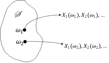
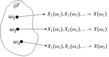
The sequence X$ _n $ maps S to the set of all sequences of real numbers, so for a fixed S, X$ _1(\omega) $,X$ _2(\omega) $,... is a sequence of real numbers.
Before looking at convergence, recall the meaning of convergence or a sequence of real numbers.
Definition $ \qquad $ A sequence of real numbers x$ _1 $,x$ _2 $,... converges to a number x ∈ R if ∀$ \epsilon $ > 0, ∃ an n$ _{\epsilon} $ ∈ N such that
If there is such an x ∈ R, we say
or
For a random sequence X$ _n $, the issue of convergence is more complicated since X$ _n $ is a function of $ \omega $ ∈ S.
First look at a motivating example.
Example $ \qquad $ Let X$ _k $ = s + W$ _k $, where s ∈ R and W$ _k $ is a random sequence with E[W$ _k $] = 0 ∀k = 1,2,.... W$ _k $ can be viewed as a noise sequence if we want to know the value of s.
Let
Then, E[Y$ _n $] = s ∀n. But Y$ _n $ is a random variable, so we cannot expect Y$ _n $ = s ∀n. However, we intuitively expect Y$ _n $ to be a better estimate of s as n increases. Does Y$ _n $ → s as n → ∞ ? If so, in what sense?
Types of Convergence
Since X$ _n(\omega) $ is generally a different sequence for very $ \omega $ ∈ S, what does it mean for X$ _n $ to converge? We will discuss different ways in which X$ _n $ can converge.
Definition $ \qquad $ X$ _n $ converges everywhere if the sequence X$ _1(\omega) $,X$ _2(\omega) $,... converges to some value X$ (\omega) $ ∀$ \omega $ ∈ S. We also call this sure convergence or convergence surely.
Notation
Definition $ \qquad $ X$ _n $ converges almost everywhere or almost surely, if X$ _n(\omega) $ → X$ (\omega) $ for some A ∈ S with P(A) = 1. Also known as convergence with probability 1.
Notation
Definition $ \qquad $ X$ _n $ converges in mean square to X if
as
Notation
Definition X$ _n $ converges in probability to X if ∀$ \epsilon $ > 0
as
Note that P(|X$ _n $ - X| > $ \epsilon $) is a sequence of real numbers.
Notation
Definition $ \qquad $ X$ _n $ converges in distribution to X if
as
Note that for a fixed x ∈ R, F$ _n $(x) is a sequence of real numbers.
Notation
We will generally assume that if X$ _n $ converges in distribution, then
or
$ f_{X_n}(x)\rightarrow f_X(x) $
as
although this is not true in every instance, as seen in the next example.
Example $ \qquad $ Let X$ _n $ have pdf
Then
Now
as
$ n\rightarrow\infty $
where
However, f$ _{Xn} $ does not converge for x ∈ (0,1).
Cauchy Criterion for Convergence
We will now discuss a method for showing that X$ _n $ → X in the mean square sense for some random variables X without knowing what X is. Frist, consider a sequence of real numbers.
Definition If x$ _n $ is a sequence of real numbers and
as
then x$ _n $ converges iff it is a Cauchy sequence. This is known as the Cauchy criterion for convergence.
The Cauchy Criterion for mean square convergence of X$ _n $ $ \qquad $ It can be shown that a random sequence X$ _n $ converges in the mean square sense iff
as
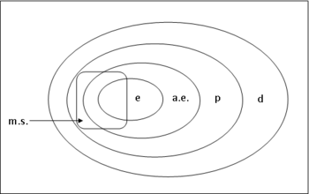
It can be shown that the following relationships between types of convergences hold:
Some Important Random Sequences
First, we need the Chebyshev Inequality:
Let X be a random variable with mean $ \mu $ and variance $ \sigma^2 $. Then,
and
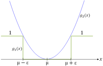
Proof $ \quad $ let
for a fixed ε > 0. Then,
and
Now consider $ \phi $(x) = g$ _2 $(x) - g$ _1 $(x)
We have that $ \phi $(x) ≥ 0 ∀x ∈ R. So,
The Laws of Large Numbers
Recall that the previous example where
where s ∈ R and E[W$ _k $] = 0. Let
Does Y$ _n $ converge to s? If so, in what sense? The laws of large numbers address this question.
Theorem $ \qquad $ The Weak Law of Large Numbers
Let X$ _n $ be a sequence of iid random variables with mean $ \mu $ and variance $ \sigma^2 $. Let
Y$ _n $ is the sample mean.
Then, for any $ \epsilon $ < 0,
as
i.e., Y$ _n $ → $ \mu $ in probability.
Proof
Using the Chebyshev Inequality, we have that
Theorem $ \qquad $ Strong Law of Large Numbers
Let X$ _n $ be a sequence of iid random variables with mean $ \mu $ and variance $ \sigma^2 $. Then
as
The proof is omitted as it is beyond the scope of this class. Nevertheless, note that the strong law of large numbers implies the weak law of large numbers.
So for example
if the W$ _k $'s are independent and have the same variance $ \sigma^2 $, then the sample mean Y$ _n $ converges to s with probability 1.
But the laws of large numbers tell us something more fundamental about our axiomatic-based probability measure. Consider a random variable X and a set A ⊂ B(R). Let X$ _1 $,X$ _2 $,... be an iid sequence of random variables with the same distribution as X. Now let
Then
The Y $ _k $'s are iid with with mean P(X ∈ A) and the relative frequency of the even {X ∈ A} is
The strong law pf large number tells us that
with probability 1 as
So with probability 1, the relative frequency approach to probability converges to the axiom-based P(X ∈ A).
The Central Limit Theorem
Let X$ _n $ be a sequence of iid random variables with finite mean $ \mu $ and variance $ \sigma^2 $. Then if
then,
as
where Z is N(0,1).
i.e.
Proof $ \qquad $ We will use the following Lemma
Lemma $ \qquad $ Let Z$ _n $ be a sequence of random variables with cdfs F$ _{Zn} $ and mgfs $ \Phi_{Zn} $(s), and let Z be a random variable with cdf F$ _Z $ and mgf $ \Phi_Z $. Then if $ \Phi_{Zn} $(s) → $ \Phi_Z $ ∀s ∈ C, then F$ _{Zn} $(z) → F$ _Z $(z) ∀z ∈ R.
So it is sufficient to show that
Consider
Now considering the case $ \mu=0 $, $ \sigma^2=1 $, we have
Let L(s) = log$ |phi_X $(s). Then, to show that
it is sufficient to show that
Will need
Now
For general $ \mu $, $ \sigma^2 $, use the result for $ \mu $ = 0, $ \sigma^2 $ = 1 with
References
- M. Comer. ECE 600. Class Lecture. Random Variables and Signals. Faculty of Electrical Engineering, Purdue University. Fall 2013.
Questions and comments
If you have any questions, comments, etc. please post them on this page


