ECE600 F13 Linear Systems with Random Inputs mhossain - Rhea

Topic 20: Linear Systems with Random Inputs

Linear Systems with Random Inputs

We will now study what happens when a random signal is the input to a linear system, or more specifically, a linear time-invariant (LTI) system. We will characterize the output is the system by finding the mean and autocorrelation functions of the output in terms of those of the input signal.

Recall that an LTI system can be characterized by its impulse response h(t).

Fig 1: An LTI system. The impulse response is the output of the system when the input is an impulse or delta function

With an arbitrary input x(t), the output of the system is x(t) * h(t).

What if the imput is a random process X(t)? Then we have the scenario depicted in figure 2.

Fig 1: X(t) is an arbitrary random process.

Then, ∀ $\omega$ ∈ S,

\begin{align}Y(t,\omega)&=X(t,\omega)\ast h(t) \\ &=\int_{-\infty}^{\infty}X(t-\alpha,\omega)h(\alpha)d\alpha \end{align}

Dropping $\omega$ from the notation,

Y(t) = X(t)\ast h(t)

We want to know E[Y(t)] and R $_{YY}$ (t $$ _1 $$ ,t $$ _2 $$ ).

First the mean:

\begin{align} E[Y(t)]&=E\left[\int_{-\infty}^{\infty}X(t-\alpha)h(\alpha)d\alpha\right] \\ &=\int_{-\infty}^{\infty}E[X(t-\alpha)]h(\alpha) \\ &=\mu_X(t)\ast h(t) \end{align}

So

\mu_Y(t) = \mu_X(t)\ast h(t)

Now R $_{YY}$ (t):

\begin{align} R_{YY}(t_1,t_2)&=E[Y(t_1)Y(t_2)] \\ &=E\left[\int_{-\infty}^{\infty}X(t_1-\alpha)h(\alpha)d\alpha \int_{-\infty}^{\infty}X(t_2-\beta)h(\beta)d\beta\right] \\ &=\underset{\mathbb R^2}{\int\int}E[X(t_1-\alpha)X(t_2-\beta)]h(\alpha)h(\beta)d\alpha d\beta \end{align}

So

R_{YY}(t_1,t_2)=\underset{\mathbb R^2}{\int\int}R_{XX}(t_1-\alpha,t_2-\beta)h(\alpha)h(\beta)d\alpha d\beta

Very often, we will assume that X(t) is WSS. What happens to $\mu_Y$ and R $_{YY}$ then?

First the mean:

\begin{align} \mu_Y(t) &= \int_{-\infty}^{\infty}\mu_X(t-\alpha)h(\alpha)d\alpha \\ &=\mu_X\int_{-\infty}^{\infty}h(\alpha)d\alpha \end{align}

So $\mu_Y$ (t) does not depend on t and

\mu_Y=\mu_X\int_{-\infty}^{\infty}h(\alpha)d\alpha

Now R $_{YY}$ : from earlier,

\begin{align} R_{YY}(t_1,t_2)&=\underset{\mathbb R^2}{\int\int}R_{XX}(t_1-\alpha,t_2-\beta)h(\alpha)h(\beta)d\alpha d\beta \\ &= \underset{\mathbb R^2}{\int\int}R_X(t_2-t_1-\beta+\alpha)h(\alpha)h(\beta)d\alpha d\beta \\ &= \underset{\mathbb R^2}{\int\int}R_X\tau-\beta+\alpha)h(\alpha)h(\beta)d\alpha d\beta \\ &=R_Y(\tau) \end{align}

for some function R $$ _Y $$ : R → R, where $\tau$ = t $$ _2 $$ - t $$ _1 $$ .

Constant $\mu_Y$ and R $_{YY}$ (t $$ _1 $$ ,t $$ _2 $$ ) = R $_Y(\tau)$ implies:

Important result: If the input of a stable LTI system is WSS, then the out put is WSS. By stable LTI system characterized by impulse response h(t) we mean that

\int_{-\infty}^{\infty}h(\alpha)d\alpha < \infty

The Power Spectrum

What is the "frequency content" of a random process X(t)?

Definition $\qquad$ The power spectral density or PSD of a WSS random process X(t) is the Fourier transform of its autocorrelation function:

S_X(\omega) =\int_{-\infty}^{\infty}R_X(\tau)e^{-i\omega\tau}d\tau

Poperties:

Since R $_X(-\tau)$ = R $_X(\tau)$ , S $_X(\omega)$ is real.

R_X(\tau) =\frac{1}{2\pi}\int_{-\infty}^{\infty}S_X(\omega)e^{i\omega\tau}d\omega

R $_X(\tau)$ real ⇒ S $_X(\omega)$ is an even function of $\omega$

Definition $\qquad$ The cross correaltion function of random processes X(t) and Y(t) is

\tilde{R}_{XY}(t_1,t_2)=E[X(t_1)Y(t_2)]

Definition $\qquad$ The random processes X(t) and Y(t) are jointly WSS if each is WSS and

\tilde{R}_{XY}(t_1,t_2)=R_{XY}(\tau)

for some R $_{XY}$ : R → R, where $\tau$ = t $$ _1 $$ - t $$ _2 $$ .

Definition $\qquad$ The cross power spectral density of two jointly WSS random process X(t) and Y(t) is

S_{XY}(\omega) = \int_{-\infty}^{\infty}R_{XY}(\tau)e^{-i\omega\tau}d\tau

Question: If X(t) is the WSS input to an LTI system with impulse response h(t), then what is the PSD of the output Y(t)?

First, write R $_Y(\tau)$ as a convolution. From before, we have that

\begin{align}R_Y(\tau)&= \int_{-\infty}^{\infty}h(\alpha) \int_{-\infty}^{\infty}h(\beta)R_X(\tau+\alpha-\beta)d\beta d\alpha \\ &= \int_{-\infty}^{\infty} h(\alpha)(h\ast R_X)(\tau+\alpha)d\alpha \end{align}

Let $\lambda = -\alpha$ . Then,

\begin{align} R_Y(\tau)&= \int_{-\infty}^{\infty}y(-\lambda)(h\ast R_X)(\tau-\lambda)d\lambda \\ &=(\tilde{h}\ast h\ast R_X)(\tau) \end{align}

where

\tilde{h} = h(-t)

Let

H(\omega) = \int_{-\infty}^{\infty}h(t)e^{-i\omega t}dt

Then

S_Y(\omega)=|H(\omega)|^2S_X(\omega) \

Also, it can be shown that

R_{XY}(\tau) = (h\ast R_X)(\tau)

So

S_{XY}(\omega) = H(\omega)S_X(\omega) \

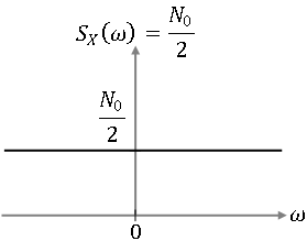
Example $\qquad$ If X(t) is white noise, zero mean, then

R_X(\tau) = \frac{N_0}{2}\delta(\tau)

\Rightarrow S_X(\omega) = \frac{N_0}{2}

Fig 3: Power spectral density S

_X(\omega)

, of a zero mean, white noise random process X(t).

Example $\qquad$ Given

h(t) = e^{-t}u(t) \

X(t) is white noise with $\mu_X$ = 0 and

R_X(\tau) =\frac{N_0}{2}\delta(\tau)

Then,

\mu_y = 0 \

and

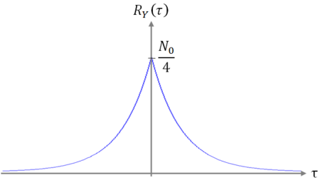
R_Y(\tau)=\frac{N_0}{4}e^{-|\tau|}

To show this,

\mu_Y = \mu_X\int_{-\infty}^{\infty}h(t)dt = 0

$H(\omega)=\frac{1}{1+i\omega}$

S_Y(\omega) = S_X(\omega)|H(\omega)|^2 = \frac{N_0/2}{1+\omega^2}

So

R_Y(\tau) = \frac{N_0}{4}e^{-|\tau|}

This result could have also been derived using

R_Y(\tau)=(\tilde{h}\ast h\ast R_X)(\tau)

Fig 4: R

_Y(\tau)

.

References

M. Comer. ECE 600. Class Lecture. Random Variables and Signals. Faculty of Electrical Engineering, Purdue University. Fall 2013.

Questions and comments

If you have any questions, comments, etc. please post them on this page

Back to all ECE 600 notes

ECE600 F13 Linear Systems with Random Inputs mhossain - Rhea

Contents

Linear Systems with Random Inputs

The Power Spectrum

References

Questions and comments

Alumni Liaison