Upper Bounds for Bayes Error
Partly based on the ECE662 Spring 2014 lecture material of Prof. Mireille Boutin.
Contents
Introduction
This lecture is dedicated to explain upper bounds for Bayes Error. In order to motivate the problem we will first discuss what Bayes rule is, and how it is used to classify continuously valued data. Then we will present the probability of error that results from using Bayes rule.
When Bayes rule is used the resulting probability of error is the smallest possible error, and therefore becomes a very important quantity to know. Although, in many cases computing this error is intractable and therefore having an upper bound to the Bayes error becomes useful. The Chernoff Bound is one such upper bound which is reasonably easy to compute in many cases. Therefore we will present this bound, and then discuss a few results that can be attained for certain types of distributions.
Bayes rule for classifying continuously valued data
Let's assume that the features $ x $ are continuously valued and that $ x \in \mathbb{R}^{N} $ . We will also assume that the data belongs to two different classes, $ \omega_1 $ and $ \omega_2 $. Then our objective is to classify the data in to these two classes.
We can classify $ x $ to be in $ \omega_1 $ if the probability of class $ 1 $ given the feature vector $ x $ is larger than the probability of class $ 2 $ given the feature vector $ x $ . Hence,
then that particular feature vector $ x $ belongs in class $ 1 $, and vise versa. Although, in many cases calculating $ \rho(\omega_i | x) $ is impossible, or extremely difficult. Therefore, we use Bayes theorem to simplify our problem.
Bayes theorem states,
Here, $ \rho(x|\omega_i) $ is the probability density of $ x $ given it belongs to class $ i $, $ Prob(\omega_i) $ known as the prior probability is the probability of class $ i $, and $ \rho(x) $ is the probability density of $ x $. Using equation (2), inequality (1) can be re-written as,
Probability of Error when using Bayes rule
When using a certain method for classifying data, it is important to know the probability of making an error, because the ultimate goal of classification is to minimize this error. When we use Bayes rule to classify data, the probability of error is,
Then using the definition of conditional probability we can rewrite this equation as,
Now let us look at an example to understand how we can write this integral in terms of $ Prob \left( \omega_1 \vert x\right) $ and $ Prob \left( \omega_1 \vert x\right) $.
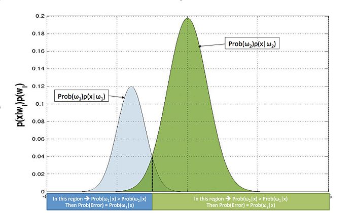
From equation (2) we know that $ Prob \left( \omega_i \vert x\right) \propto \rho(x|\omega_i) Prob(\omega_i) $, and therefore $ \rho(x|\omega_i) Prob(\omega_i) $ and $ Prob \left( \omega_i \vert x\right) $ will have the same shape. Therefore, we plot $ \rho(x|\omega_1) Prob(\omega_1) $ and $ \rho(x|\omega_2) Prob(\omega_2) $ on the same plot as shown in Figure 1.
From this we can see that errors happen in the regions where the two curves intersect. For example, if we consider a point in the region where $ \rho(x|\omega_1) Prob(\omega_1) $ and $ \rho(x|\omega_2) Prob(\omega_2) $ intersect, and $ \rho(x|\omega_1) Prob(\omega_1) \geq \rho(x|\omega_2) Prob(\omega_2) $, it will be classified as Class $ 1 $.
Now since $ Prob \left( \omega_i \vert x\right) \propto \rho(x|\omega_i) Prob(\omega_i) $, our expression for the probability of error can be written as,
It is important to note that the above example is a trivial case when there is just one intersection between the curves. There can be any number of intersections in the general case, but even still the same equation holds. In this case the probability of error will be the summation of the integrals over the lesser of the $ Prob \left( \omega_i \vert x \right) $'s in the different regions, which once more is given by equation (6).
By using Bayes Theorem, we can simplify further so that,
In most cases solving either integral is intractable because these could be integrals in large dimensions. Therefore the need for an approximate answer becomes necessary.
Of course our goal will always be to get the smallest possible probability of error. Although, we know Bayes error is almost impossible to calculate in many cases. So instead what we can do is find an upper bound to the Bayes error.
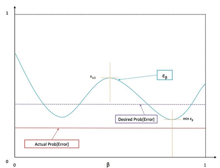
For example let us assume that we want the probability of error to be lower than $ 0.05 $. Now if we find an upper bound to Bayes error that is less than $ 0.05 $, we definitely know that Bayes error is less than $ 0.05 $. In the next section we will explore a single parameter family of upper bounds to Bayes error, the 'Chernoff Bound.
Chernoff Bound
To formulate the Chernoff bound we use the following mathematical property: If $ a,b \in \mathbb{R}_{\geq 0} $, and $ 0 \leq \beta \leq 1 $ then,
Since equation (6) has probabilities and they are non-negative, we can use inequality (7) and get the following upper bound for the probability of error,
This family of upper bounds parameterized by $ \beta $ is known as the Chernoff bound ($ \varepsilon_{\beta} $).

If needed it is possible to find the smallest error bound by solving,
Although, this is not necessarily an easy problem to solve, because the optimization problem might not be convex and might have local minimums. For the purpose of evaluating a classification method one can try with different values for $ \beta $, and compare the least value of $ \varepsilon_{\beta} $ with the desired error probability.
In the special case where $ \beta = \frac{1}{2} $, the Chernoff bound, $ \varepsilon_{\frac{1}{2}} $, is known as the Bhattacharyya bound.
Chernoff bound for Normally distributed data
When $ \rho (x\vert \omega_i) $ is Normally distributed and has mean $ \mu_i $ and covariance $ \Sigma_i $, the Chernoff bound has the following closed form solution,
where,
$ f(\beta) = \frac{\beta(1-\beta)}{2} (\mu_2 - \mu_1)^t \left[ \beta \Sigma_1 + (1-\beta) \Sigma_2 \right]^{-1}(\mu_2 - \mu_1)+ \frac{1}{2} \ln \left( \frac{\vert \beta \Sigma_1 + (1-\beta) \Sigma_2 \vert}{\vert \Sigma_1 \vert^{\beta} \vert \Sigma_2 \vert^{1-\beta}} \right). $
In this case the Bhattacharyya bound becomes,
where,
Notice that if$ \mu_2=\mu_1 $, then the first term in $ f \left(\frac{1}{2}\right) $ disappears. This term basically describes the separability due to the "distance" between the two mean values. Here the "distance" is described by metric defined by the matrix $ \left[ \frac{\Sigma_1 + \Sigma_2 }{2}\right]^{-1} $.
The second term disappears if the covariance matrices are equal, i.e. $ \Sigma_1 = \Sigma_2 $. Also, in this case it can be shown that, $ \varepsilon_{\frac{1}{2}} = \varepsilon_{min} $.
Proof: We want to minimize $ \varepsilon_{\beta} $ , which means we want maximize $ f(\beta) $.
Since this is convex in $ \beta $ we know that there is only one maximum and that maximum is the global maximum. So we take the derivative w.r.t. $ \beta $, and set it equal to zero to find the maximum.
if $ \mu_1 = \mu_2 $, then $ f(\beta) =0 $, and $ \varepsilon_{\beta} = constant $. This means $ \varepsilon_{min} = \varepsilon_{\frac{1}{2}} $.
if $ \mu_1 \neq \mu_2 $, then the $ \beta $ that maximizes $ f(\beta) $ is $ \beta = \frac{1}{2} $. Then $ \varepsilon_{min} = \varepsilon_{\frac{1}{2}} $ .
Summary and Conclusions
In this lecture we have shown that the probability of error ($Prob \left[ Error \right] $) when using Bayes error, is upper bounded by the Chernoff Bound. Therefore,
for $ \beta \in \left[ 0, 1 \right] $.
When $ \beta =\frac{1}{2} $ then $ \varepsilon_{\frac{1}{2}} $ in known as the Bhattacharyya bound.
References
[1]. Duda, Richard O. and Hart, Peter E. and Stork, David G., "Pattern Classication (2nd Edition)," Wiley-Interscience, 2000.
[2]. Mireille Boutin, "ECE662: Statistical Pattern Recognition and Decision Making Processes," Purdue University, Spring 2014.
Questions and comments
If you have any questions, comments, etc. please post them On this page.


