| Line 35: | Line 35: | ||
[[Image:Cos2D_withDC.png|left|800px]] | [[Image:Cos2D_withDC.png|left|800px]] | ||
Note that the added DC term of 1 shows up in the CSFT as an impulse at the origin (u=0, v=0).<br><br> | Note that the added DC term of 1 shows up in the CSFT as an impulse at the origin (u=0, v=0).<br><br> | ||
| − | Now let's combine two 2D cosine waves: | + | '''Now let's combine two 2D cosine waves:''' |
[[Image:CosTwice.png|left|800px]] | [[Image:CosTwice.png|left|800px]] | ||
| − | Can you see all five components? | + | Can you see all five components? There is a small component at the origin (due to the 0.2 DC term)! |
---- | ---- | ||
<br><br> | <br><br> | ||
Revision as of 08:31, 26 November 2009
Spectral Analysis of 2D Signals (December 1, 2009)
Here, I will describe and explain the basics behind analyzing the spectrum of 2-D signals - principally images! - Ryan Scheidt
Spectral analysis of two-dimensional (2D) signals is not much different from the one-dimensional (1D) FFT [Fast Fourier Transform - see [1]] that we are (more) accustomed to. The only difference is that our signals are now represented in one more plane. We can think of this difference (1D vs. 2D) as the difference between, say, a one-dimensional longitudinal wave in a slinky (like this: [2]), versus a two-dimensional wave from a trampoline (e.g. drop a baseball in the center (or given any other excitation), and the wave will propagate in both x and y-directions ([3]).
For those familiar with the properties of the 1D Fourier Transform (FT), the 2-D Continuous-Space Fourier Transform (CSFT) [see [4] for a reference] is an intuitive extension of the 1D properties. The following Rhea link shows some of these properties: [5].
Now let's look at the spectral analysis of some elementary 2D signals.
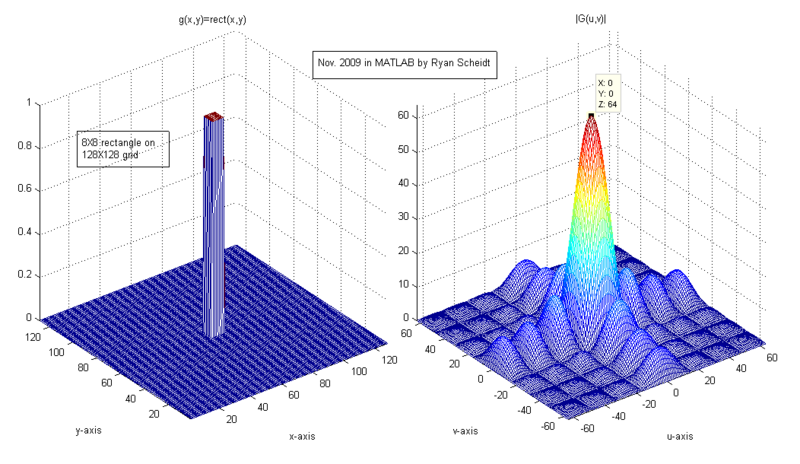
We'll start with the 2-dimensional rect(*) signal. Here's the 2-dimensional rect(x,y) function and its CSFT:
(Note: click on any of the following images and then click on the "Full resolution" hyperlink to see the full image.)
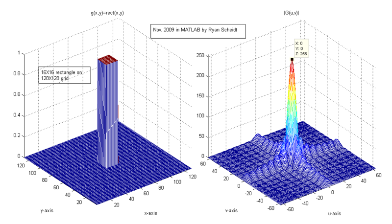
Now let's make the "rectangle" a little bit bigger: 16X16. We'll watch what happens to the frequency of the 2-dimensional sinc function:
This is exactly what was expected. Remember, that when we double the width of a 1D rect(x) function, the corresponding sinc(f) has twice the height and twice the frequency. In two dimensions, the corresponding will thus be quadrupled in height (multiplied by two twice), with twice the frequency.
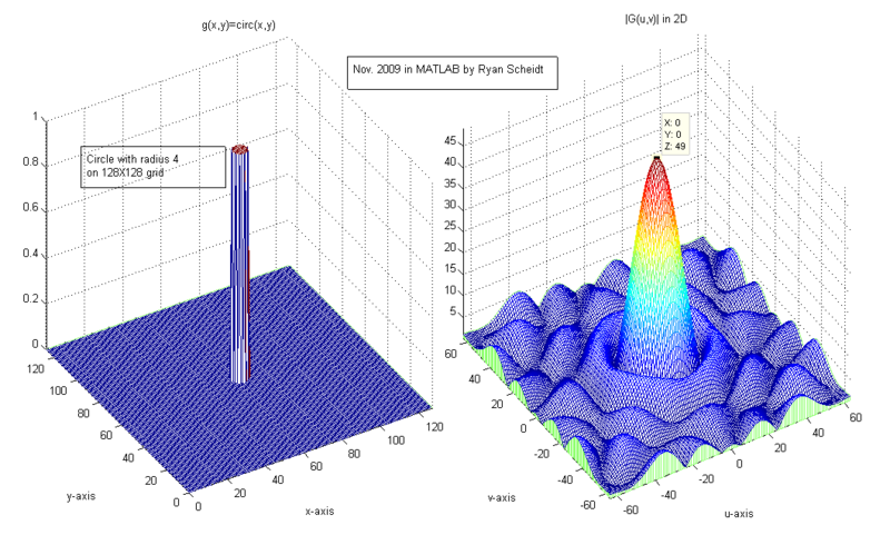
Now let's look at the 2D circ(*) function. Here's the 2-dimensional circ(x,y) function and its CSFT:
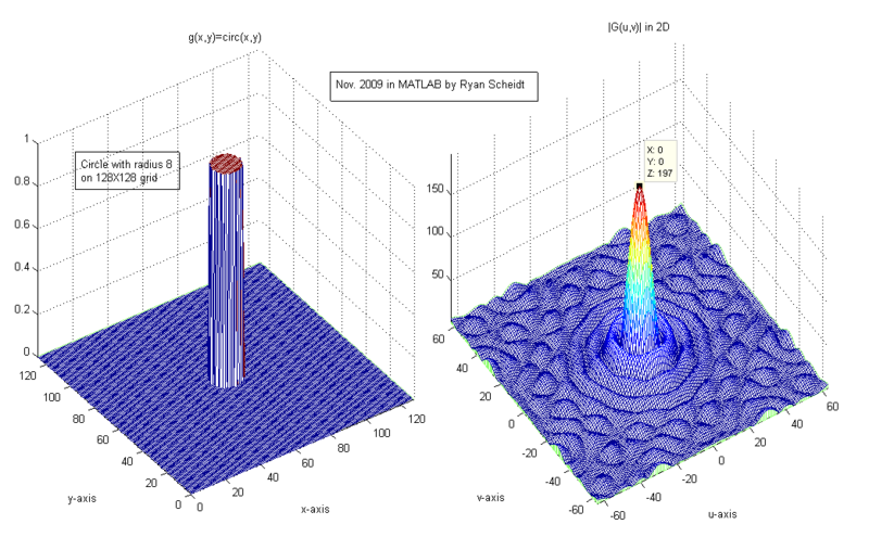
Now let's make the "circle" a little bit larger with a radius of 8. We'll watch what happens to the frequency of the 2-dimensional jinc function:
Note that both the frequency and magnitude of the jinc(u,v) also went up (more precisely: magnitude quadrupled and frequency doubled, just like the sinc(u,v) as done previously).
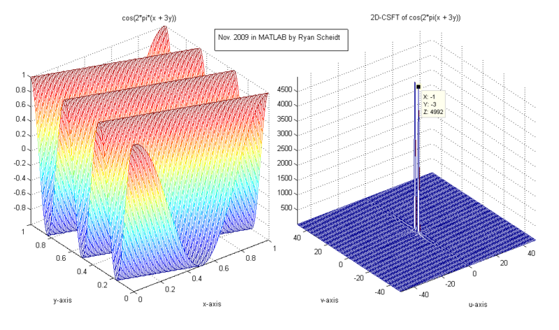
Now let's look at the 2D cos(*) function. Here's a 2-dimensional cos(x,y) function and its CSFT:
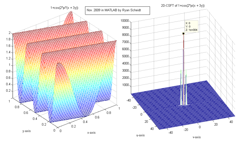
Now let's add a DC component and watch what happens to the CSFT components:
Note that the added DC term of 1 shows up in the CSFT as an impulse at the origin (u=0, v=0).
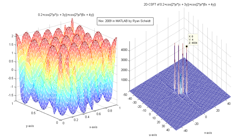
Now let's combine two 2D cosine waves:
Can you see all five components? There is a small component at the origin (due to the 0.2 DC term)!
Now let's look at images briefly.
The following image, commonly referred to as "Lena" (sometimes also "Lenna"), is a famous image utilized in standard image processing algorithms and testing. The background behind this image is quite interesting. Here are some links for the interested reader: [6], [7]
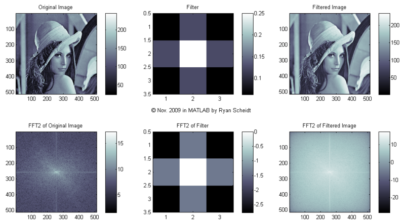
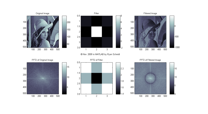
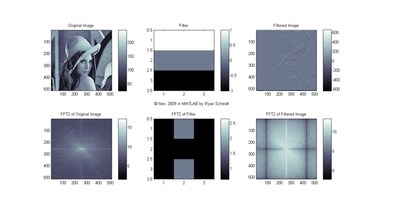
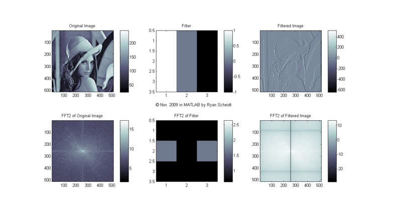
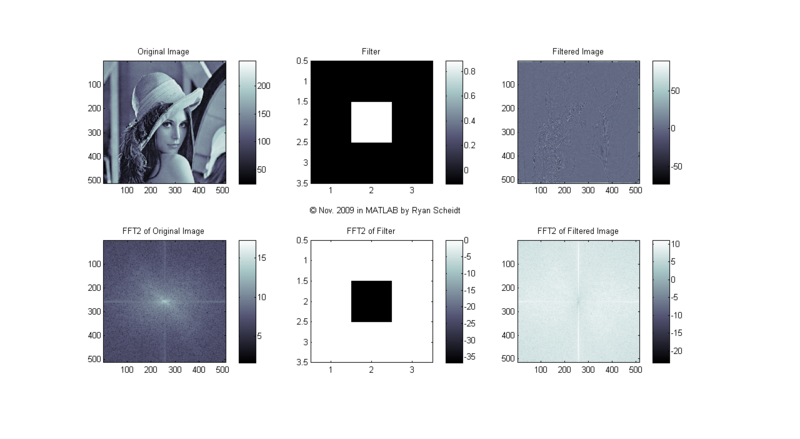
Let's look at what the 2D FFT of Lena looks like. We will look at some simple 3X3 filters that are then convolved with the original image to create a filtered image. [Here is an excellent webpage showing how 2D convolution works: [8]]
The following pictures show the original image (Lena), the image of the filter, and the filtered image (done with conv2). MATLAB m-files available upon request.
The colormaps to the right of each image show the corresponding values for each shade of gray (i.e. continuum from white to black). Each image is "normalized to 256 values" so that for each pixel, the lowest values (even if negative) are mapped to 0 (black) and the highest values are mapped to 255 (white).
Let's start with the filter = 1/16*[1 2 1; 2 4 2; 1 2 1], commonly referred to as an "average filter":
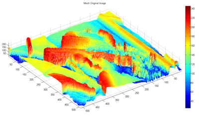
Can you tell that the filtered image is "smoothed"? Let's look at the images as 3-dimensional projections for easier visualization (via MATLAB's mesh command). First the original image:
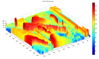
Notice that the following filtered image has much more gradual color gradations (e.g. the red "lingers around longer" and there is less blue; this is because this filter acts as a low pass filter, removing high frequency components!):
