Material Summary
In this lecture we deal on Continuous signals, Linearity, and of course, some MATLAB.
Continuous Signal
Continuous signal is a signal that varies with time, and can be represented as a function of time, x(t).
Examples : Sin waves, Sound, AC/ DC currents
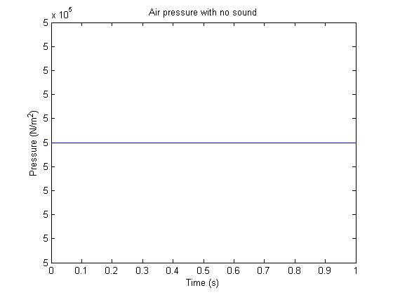
Take sound as an example, with absence of sound, the air pressure, x(t) is a constant value, approximately $ 10^5 N/m^2 $.
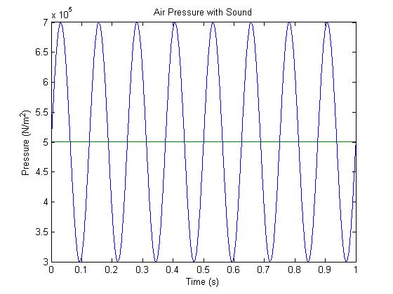
Thus, if there's sound, there would be varioation of air pressure about the atmospheric pressure.
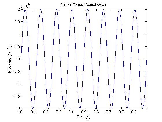
As the pressure varies around x(t) = $ 10^5 $, we gauge shift the graphs such that it is pulled down to 0.
Using any examples, one can notice that while the sound's amplitude increases, the louder the voice is. In the other hand, if the frequency increases, the higher the pitch is.
This is quite noticable if you had a sound editing program. Observe the frequency change when the pitch changes, and the amplitude change when the loudness changes.
Matlab
A very simple example of matlab code to produce the note "A" :
delta = 0.00005;
t = 0:delta:5 ;
y = sin(2*pi*440*t);
sound (y, 1/delta);
Linearity
Feedback
Did the second lecture make sense? Please write your feedback here.


